Statistics
Statistics are a feature of resistics meant to provide more insight into the data and more options for masking noisy or bad time windows. They are calculated out for each evaluation frequency at each decimation level. As statistics are calculated out for each evaluation frequency, variation in statistic values can be viewed across time and evaluation frequency.
There are a number of built in statistics and an intention to support custom statistics in the future. The following section covers the usage of statistics. For more information about the available statistics and their meanings, please refer to Statistics and Remote statistics.
As normal, begin with loading the project.
1 2 3 4 5 | from datapaths import projectPath, imagePath
from resistics.project.io import loadProject
# need the project path for loading
projData = loadProject(projectPath)
|
The next step is to get a list of the resistics built in statistics. These come in two flavours:
Statistics that are calculated for a single site
Statistics that incorporate a remote reference site
7 8 9 10 | # get default statistic names
from resistics.statistics.utils import getStatNames
stats, remotestats = getStatNames()
|
Note
For statistics that incorporate a remote reference, please see Remote reference statistics.
Statistics are calculated using the calculateStatistics() method of the project statistics module. By default, this does not calculate all available statistics but by passing the stats keyword, the statistics to calculate can be specified.
12 13 14 15 | # calculate statistics
from resistics.project.statistics import calculateStatistics
calculateStatistics(projData, stats=stats)
|
The single site statistics which are calculated by default are coherence and transfer function values. There are two ways to manually specify the statistics to calculate. These are:
By providing the stats keyword with a list of statistics as above
By defining the statistics to use in a configuration file
Note
Calculating statistics is quite demanding on compute. If the time series data quality is generally good, it is sufficient to calculate out only window coherence or window coherence and impedance tensor. In more complex situations, some of the other statistics may add value. For more on the different statistics available on what they mean, please see Statistics and Remote statistics.
Once calculated, statistics are stored in the following location:
exampleProject
├── calData
├── timeData
│ └── site1
| |── dataFolder1
│ |── dataFolder2
| |── .
| |── .
| |── .
| └── dataFolderN
├── specData
│ └── site1
| |── dataFolder1
| | |── dec8_5
| | └── spectra
| |
│ |── dataFolder2
| | |── dec8_5
| | └── spectra
| |── .
| |── .
| |── .
| └── dataFolderN
| |── dec8_5
| └── spectra
├── statData
│ └── site1
| |── dataFolder1
| | |── dec8_5
| | | |── coherence
| | | |── .
| | | |── .
| | | |── .
| | | |── resPhase
| | | └── transferFunction
| | └── spectra
| | |── coherence
| | |── .
| | |── .
| | |── .
| | |── resPhase
| | └── transferFunction
| |
│ |── dataFolder2
| | |── dec8_5
| | | |── coherence
| | | |── .
| | | |── .
| | | |── .
| | | |── resPhase
| | | └── transferFunction
| | └── spectra
| | |── coherence
| | |── .
| | |── .
| | |── .
| | |── resPhase
| | └── transferFunction
| |── .
| |── .
| |── .
| └── dataFolderN
| |── dec8_5
| | |── coherence
| | |── .
| | |── .
| | |── .
| | |── resPhase
| | └── transferFunction
| └── spectra
| |── coherence
| |── .
| |── .
| |── .
| |── resPhase
| └── transferFunction
├── maskData
├── transFuncData
├── images
└── mtProj.prj
Every statistic is indexed by:
The site
The time series measurement directory
The spectra directory
The name of the statistic
When statistics are written out, they are written out with a comments file detailing the processing sequence of the data. An example comments file is shown below:
1 2 3 4 5 6 7 8 9 10 11 12 13 14 15 16 17 18 19 20 21 22 23 24 25 26 27 28 29 30 31 32 33 34 35 36 37 38 39 | Unscaled data 2012-02-10 11:05:00 to 2012-02-10 11:24:59.999756 read in from measurement E:\magnetotellurics\code\resisticsdata\tutorial\tutorialProject\timeData\site1\meas_2012-02-10_11-05-00, samples 0 to 4915199
Sampling frequency 4096.0
Scaling channel Ex with scalar -0.000112591 to give mV
Dividing channel Ex by electrode distance 0.08 km to give mV/km
Scaling channel Ey with scalar -0.000112512 to give mV
Dividing channel Ey by electrode distance 0.091 km to give mV/km
Scaling channel Hx with scalar -0.00360174 to give mV
Scaling channel Hy with scalar -0.00360038 to give mV
Scaling channel Hz with scalar -0.0036007 to give mV
Remove zeros: False, remove nans: False, remove average: True
---------------------------------------------------
Calculating project spectra
Using default configuration
Channel Ex not calibrated
Channel Ey not calibrated
Channel Hx calibrated with calibration data from file E:\magnetotellurics\code\resisticsdata\tutorial\tutorialProject\calData\Hx_MFS06365.TXT
Channel Hy calibrated with calibration data from file E:\magnetotellurics\code\resisticsdata\tutorial\tutorialProject\calData\Hy_MFS06357.TXT
Channel Hz calibrated with calibration data from file E:\magnetotellurics\code\resisticsdata\tutorial\tutorialProject\calData\Hz_MFS06307.TXT
Decimating with 7 levels and 7 frequencies per level
Evaluation frequencies for this level 1024.0, 724.0773439350246, 512.0, 362.0386719675123, 256.0, 181.01933598375615, 128.0
Windowing with window size 2048 samples and overlap 512 samples
Time data decimated from 4096.0 Hz to 512.0 Hz, new start time 2012-02-10 11:05:00, new end time 2012-02-10 11:24:59.998047
Evaluation frequencies for this level 90.50966799187808, 64.0, 45.25483399593904, 32.0, 22.62741699796952, 16.0, 11.31370849898476
Windowing with window size 512 samples and overlap 128 samples
Time data decimated from 512.0 Hz to 64.0 Hz, new start time 2012-02-10 11:05:00, new end time 2012-02-10 11:24:59.984375
Evaluation frequencies for this level 8.0, 5.65685424949238, 4.0, 2.82842712474619, 2.0, 1.414213562373095, 1.0
Windowing with window size 512 samples and overlap 128 samples
Time data decimated from 64.0 Hz to 8.0 Hz, new start time 2012-02-10 11:05:00, new end time 2012-02-10 11:24:59.875000
Time data decimated from 8.0 Hz to 4.0 Hz, new start time 2012-02-10 11:05:00, new end time 2012-02-10 11:24:59.750000
Evaluation frequencies for this level 0.7071067811865475, 0.5, 0.35355339059327373, 0.25, 0.17677669529663687, 0.125, 0.08838834764831843
Windowing with window size 512 samples and overlap 128 samples
Spectra data written out to E:\magnetotellurics\code\resisticsdata\tutorial\tutorialProject\specData\site1\meas_2012-02-10_11-05-00\spectra on 2019-10-05 19:18:01.917505 using resistics 0.0.6.dev2
---------------------------------------------------
Reading spectra data in path E:\magnetotellurics\code\resisticsdata\tutorial\tutorialProject\specData\site1\meas_2012-02-10_11-05-00\spectra
Using default configuration
Calculating statistic: coherence
Statistic components: cohExHx, cohExHy, cohEyHx, cohEyHy
Statistic data for statistic coherence written to E:\magnetotellurics\code\resisticsdata\tutorial\tutorialProject\statData\site1\meas_2012-02-10_11-05-00\spectra on 2019-10-05 21:29:55.492691 using resistics 0.0.6.dev2
---------------------------------------------------
|
To calculate statistics for a different spectra directory, either the specdir keyword can be specified in the call to calculateStatistics() or the specdir can be defined in a configuration file. For more information about using configuration files, see Using configuration files.
Statistics can be calculated again, but this time using a configuration file. The project needs to be loaded again with the configuration file in order to do this.
17 18 19 20 21 | # calculate statistics for a different spectra directory
# load the project with the tutorial configuration file
projData = loadProject(projectPath, configFile="tutorialConfig.ini")
projData.printInfo()
calculateStatistics(projData, stats=stats)
|
Statistic data can be read in using the getStatisticData() method of the project statistics module. As stated earlier, statistic data is indexed by site, measurement directory, spectra directory and statistic name. These have to be provided to getStatisticData(). However, if the specdir keyword is not provided, getStatisticData() will check if specdir is defined in the configuration file. If not, it will revert to the default configuration (and spectra directory). Additionally, the decimation level to read in has to be specified. Below is an example.
23 24 25 26 27 28 29 | # to get statistic data, we need the site, the measurement and the statistic we want
from resistics.project.statistics import getStatisticData
# coherence statistic data
statData = getStatisticData(
projData, "site1", "meas_2012-02-10_11-30-00", "coherence", declevel=0
)
|
The getStatisticData() method returns a StatisticData object. Statistic data is another data object similar to ProjectData, SiteData, TimeData or SpectrumData.
There are multiple view methods in StatisticData. These are:
view(), which plots the statistic value against timehistogram(), which plots a histogram of the statisticcrossplot(), which plots crossplots of the statistic componentsdensityplot(), which plots 2-D histograms (density plots) of the statistic components
Examples of using these methods to view statistic values and variation are shown below:
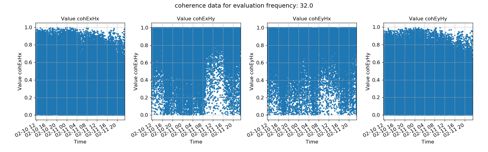
30 31 32 33 34 35 36 37 38 39 40 41 42 43 44 45 46 | # view statistic value over time
fig = statData.view(0)
fig.savefig(imagePath / "usingStats_statistic_coherence_view")
# view statistic histogram
fig = statData.histogram(0)
fig.savefig(imagePath / "usingStats_statistic_coherence_histogram")
# view statistic crossplot
fig = statData.crossplot(0, crossplots=[["cohExHy", "cohEyHx"], ["cohExHx", "cohEyHy"]])
fig.savefig(imagePath / "usingStats_statistic_coherence_crossplot")
# view statistic density plot
fig = statData.densityplot(
0,
crossplots=[["cohExHy", "cohEyHx"], ["cohExHx", "cohEyHy"]],
xlim=[0, 1],
ylim=[0, 1],
)
fig.savefig(imagePath / "usingStats_statistic_coherence_densityplot")
|
These produce the following plots:
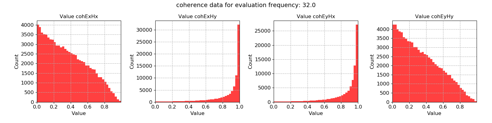
Coherence data plotted for evaluation frequency 32 Hz using the histogram() method
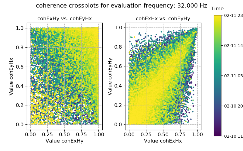
Coherence data plotted for evaluation frequency 32 Hz using the crossplot() method
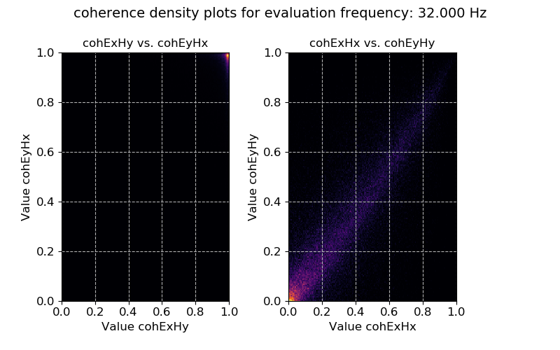
Coherence data plotted for evaluation frequency 32 Hz using the densityplot() method
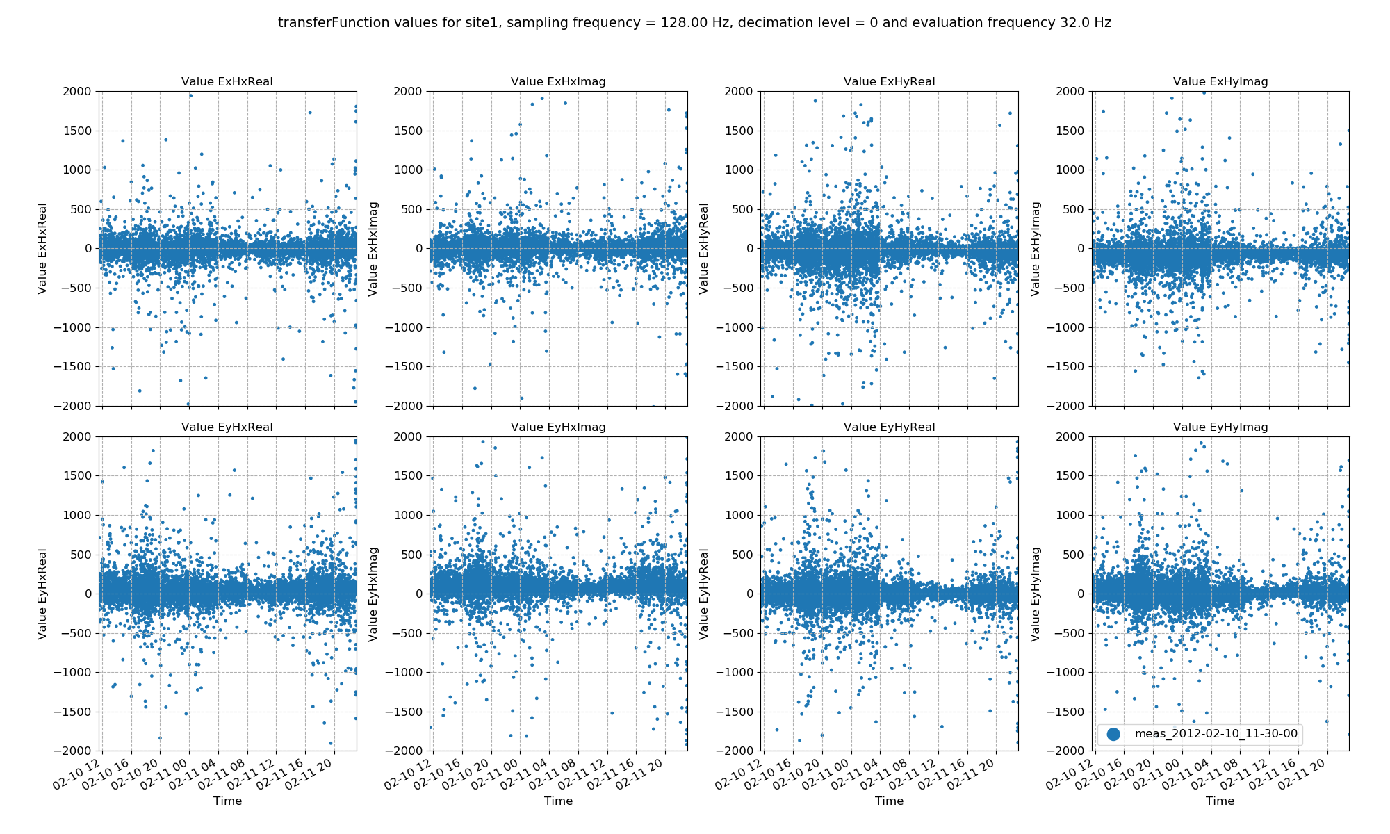
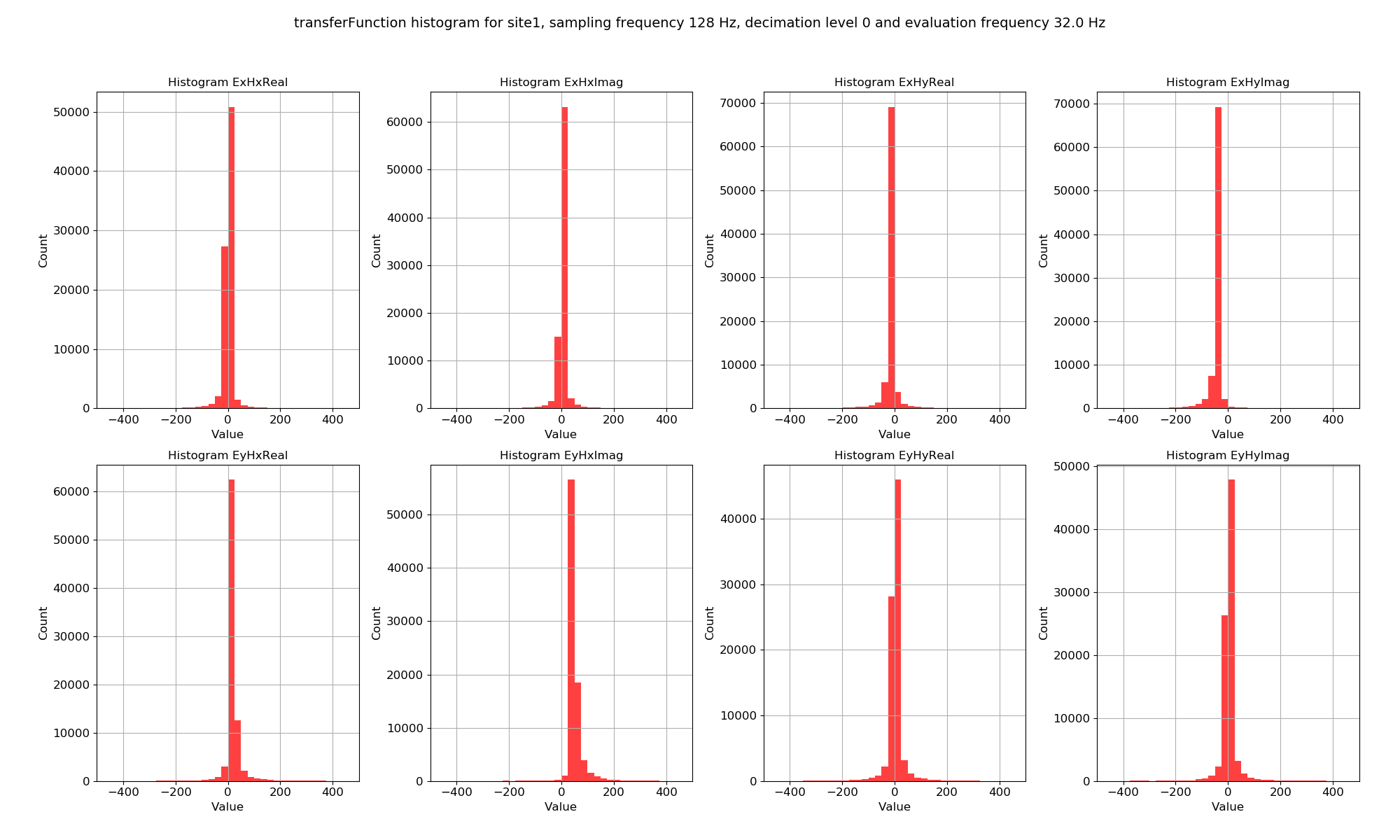
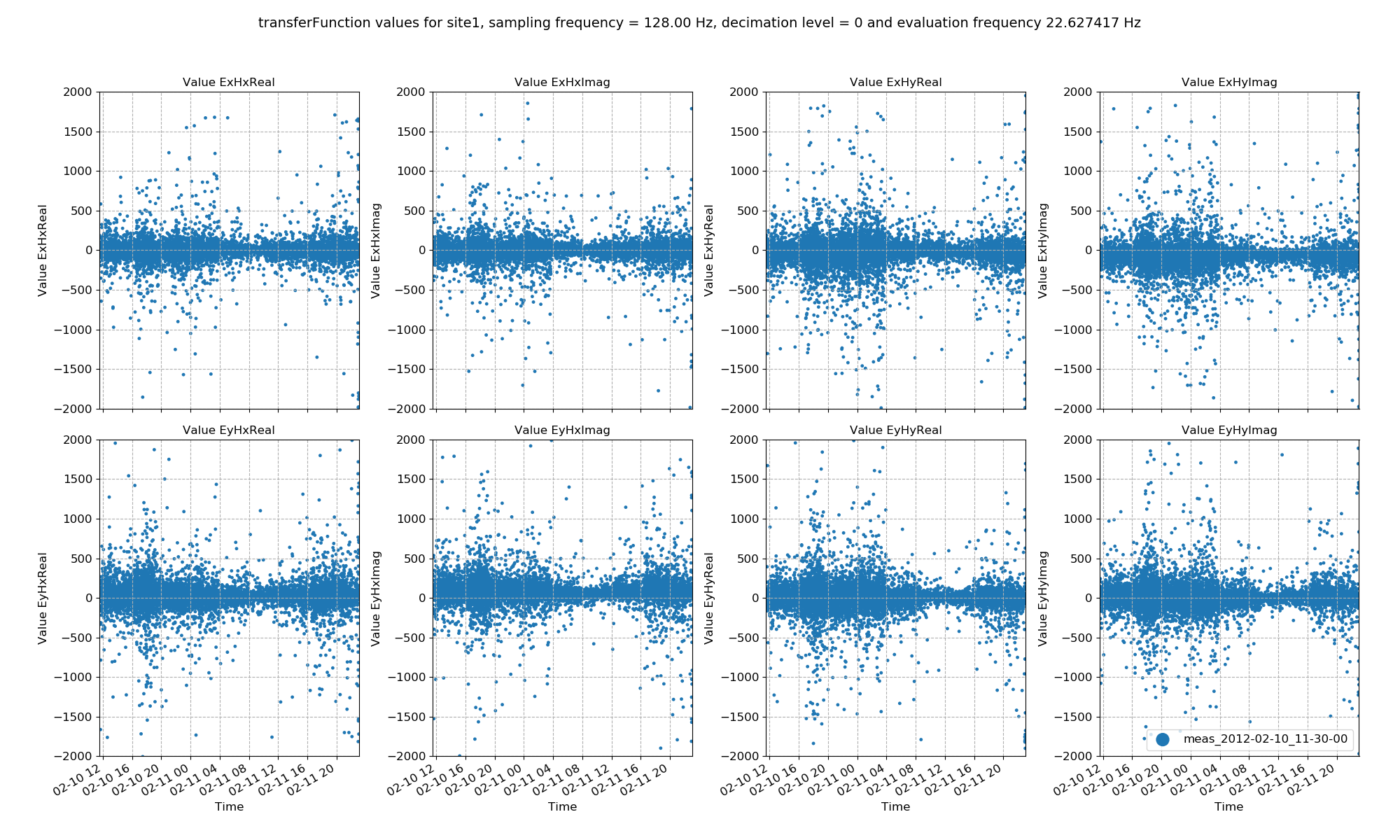
In the above case, the coherence statistic was read in. Another statistic is the transfer function calculated on a window-by-window basis. The statistic data for this can be read in and plotted in a similar way.
48 49 50 51 52 53 54 55 56 57 58 59 60 61 62 63 64 65 66 67 68 69 70 71 72 73 74 75 76 77 78 79 80 81 82 83 | # transfer function statistic data
statData = getStatisticData(
projData, "site1", "meas_2012-02-10_11-30-00", "transferFunction", declevel=0
)
# view statistic value over time
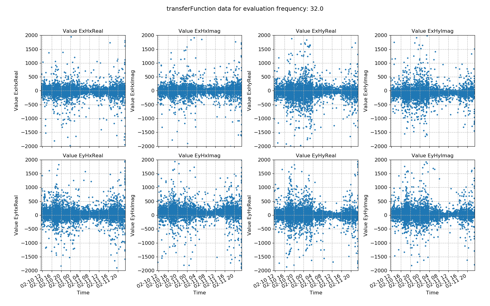
fig = statData.view(0, ylim=[-2000, 2000])
fig.savefig(imagePath / "usingStats_statistic_transferfunction_view")
# view statistic histogram
fig = statData.histogram(0, xlim=[-500, 500])
fig.savefig(imagePath / "usingStats_statistic_transferfunction_histogram")
# view statistic crossplot
fig = statData.crossplot(
0,
crossplots=[
["ExHxReal", "ExHxImag"],
["ExHyReal", "ExHyImag"],
["EyHxReal", "EyHxImag"],
["EyHyReal", "EyHyImag"],
],
xlim=[-2500, 2500],
ylim=[-2500, 2500],
)
fig.savefig(imagePath / "usingStats_statistic_transferfunction_crossplot")
# view statistic densityplot
fig = statData.densityplot(
0,
crossplots=[
["ExHxReal", "ExHxImag"],
["ExHyReal", "ExHyImag"],
["EyHxReal", "EyHxImag"],
["EyHyReal", "EyHyImag"],
],
xlim=[-60, 60],
ylim=[-60, 60],
)
fig.savefig(imagePath / "usingStats_statistic_transferfunction_densityplot")
|
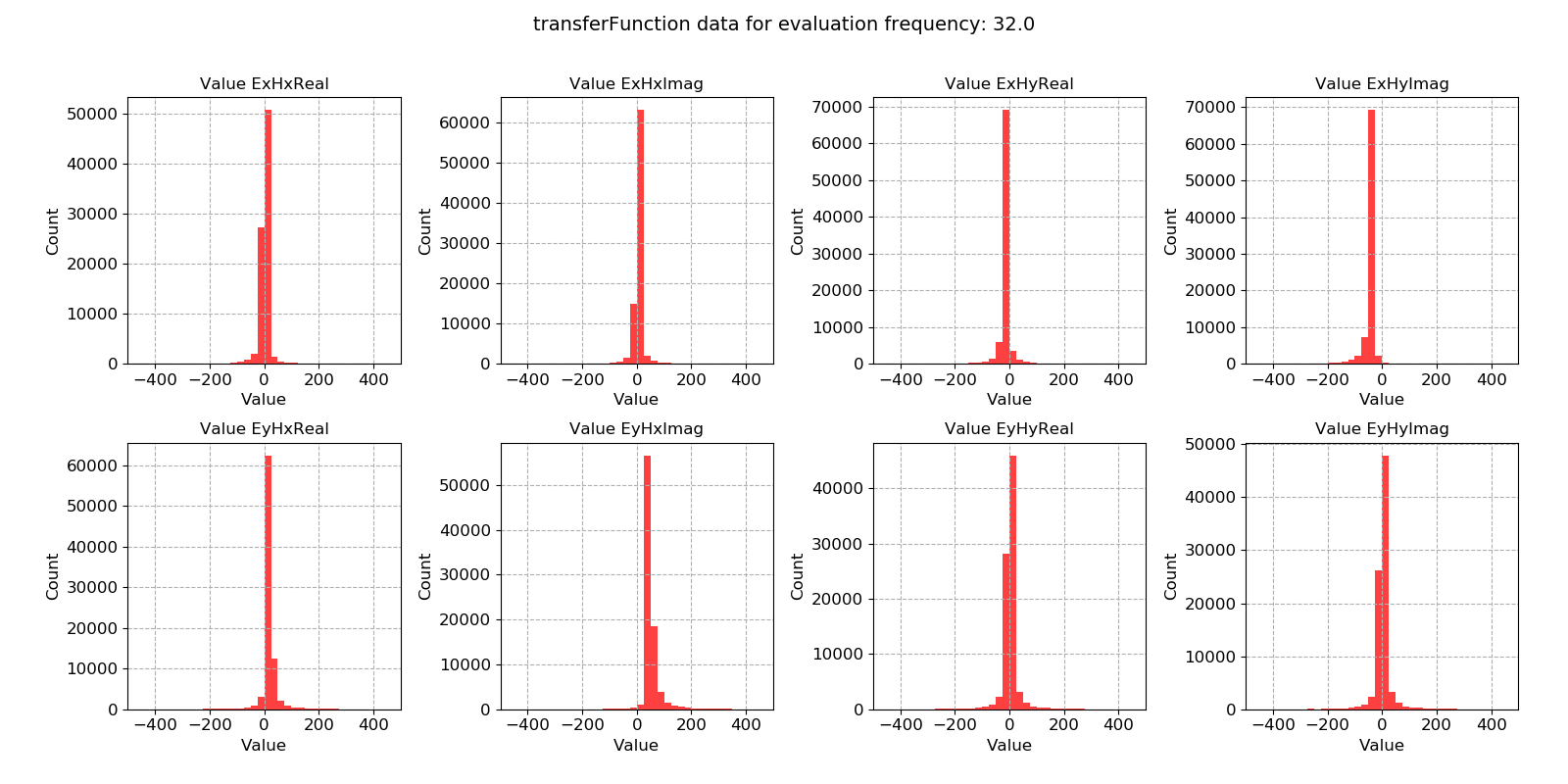
Transfer function data plotted for evaluation frequency 32 Hz using the histogram() method
The next example is the crossplot for the transfer function statistic. This make more intuitive sense than the coherence crossplot above, as it allows the plotting of the transfer function data on the complex plane.
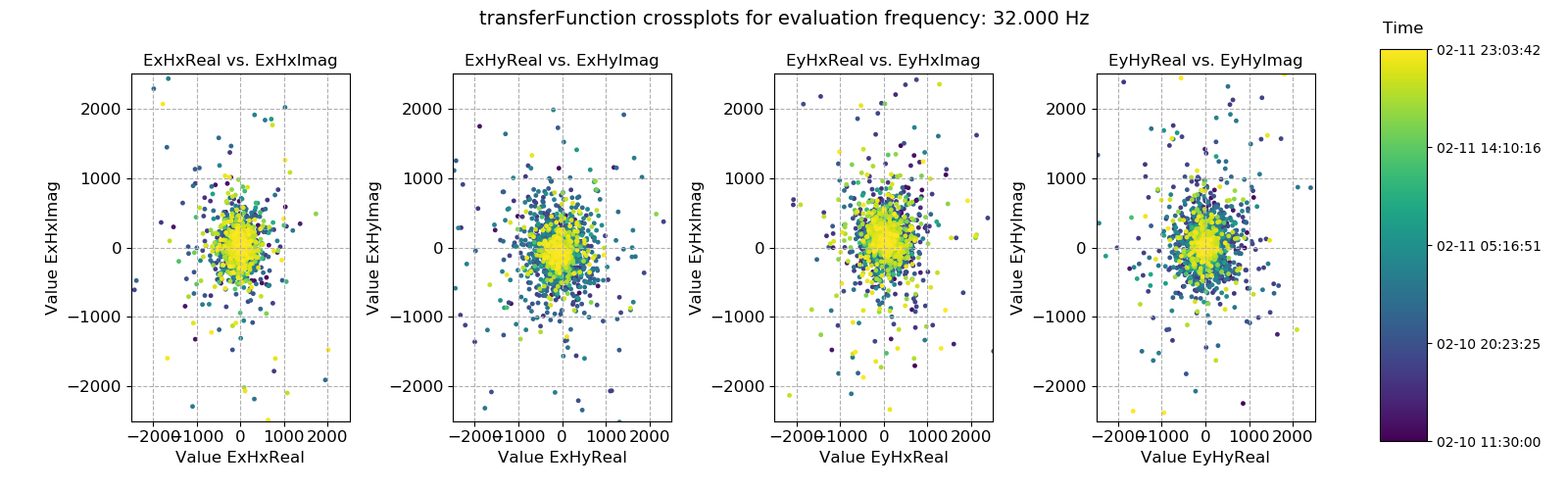
Transfer function data plotted for evaluation frequency 32 Hz using the crossplot() method
The crossplot can be used to show the scatter of the window-by-window transfer function estimates on the complex plane. Another way to look at this data is using density plots (2-D histograms), which can be achieved using the densityplot().
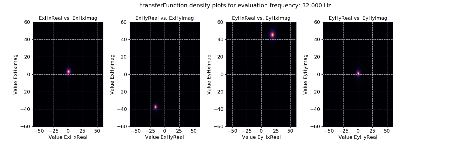
Transfer function data plotted for evaluation frequency 32 Hz using the densityplot() method. This view actually shows that the window-by-window estimates of the transfer function are actually densely clustered around the highlighted points and much more consistent than suggested by simply viewing using the crossplot() method.
In all of these cases, a 0 is being passed to the plotting methods. This 0 is the evaluation frequency index for that decimation level. Changing it will plot a different evaluation frequency.
Note
The evaluation frequency index starts from 0 and goes to the number of evaluation frequencies per decimation level - 1. So if there are 7 evaluation frequencies per decimation level, the evaluation frequency indices will be 0, 1, 2, 3, 4, 5, 6.
Evaluation frequency and decimation level indices will be covered in more detail further down.
85 86 87 | # look at the next evaluation frequency
fig = statData.view(1, ylim=[-2000, 2000])
fig.savefig(imagePath / "usingStats_statistic_transferfunction_view_eval1")
|
Statistics across time series measurements
The above examples were reading in statistic data for a single measurement. However, in many cases, the statistics over all the time series measurements of a certain sampling frequency in a site are of more interest. In order to plot and view these, the methods available in the project statistics module will be more useful. The project module statistics has four plotting methods:
These do much the same as the methods available in the class StatisticData, however, they will bring together all the statistics in a site for measurements of a given sampling frequency.
Note
For the tutorial project, there is only a single measurement at 128 Hz and a single measurement at 4096 Hz, meaning that this is not the best example of the functionality. For more interesting examples, please see Statistic plotting in the cookbook.
For example, statistic value variation across time can be plotted using viewStatistic():
88 89 90 91 92 93 94 95 96 97 98 99 100 101 |
# plot statistic values in time for all data of a specified sampling frequency in a site
from resistics.project.statistics import viewStatistic
# statistic in time
fig = viewStatistic(
projData,
"site1",
128,
"transferFunction",
ylim=[-2000, 2000],
save=False,
show=False,
)
|
This produces the plot below:
Transfer function data plotted for all time series measurements of a given sampling frequency in a site using the viewStatistic()
Statistic histograms over all time series measurements of a specified sampling frequency in a site can be plotted in a similar way.
103 104 105 106 107 108 109 110 |
# plot statistic histogram for all data of a specified sampling frequency in a site
from resistics.project.statistics import viewStatisticHistogram
# statistic histogram
fig = viewStatisticHistogram(
projData, "site1", 128, "transferFunction", xlim=[-500, 500], save=False, show=False
)
|
Transfer function data plotted for all time series measurements of a given sampling frequency in a site using the viewStatisticHistogram()
Recall, statistic values are calculated on an evaluation frequency basis. Currently, 32 Hz has been plotted, but other evaluation frequencies can be plotted by using the declevel and eFreqI keywords`.
Important
The meaning of declevel (decimation level index) and eFreqI (evaluation frequency index) are best demonstrated with an example.
Consider the evaluation frequencies in this set up using 8 decimation levels and 5 evaluation frequencies per level with a data sampling frequency of 128 Hz:
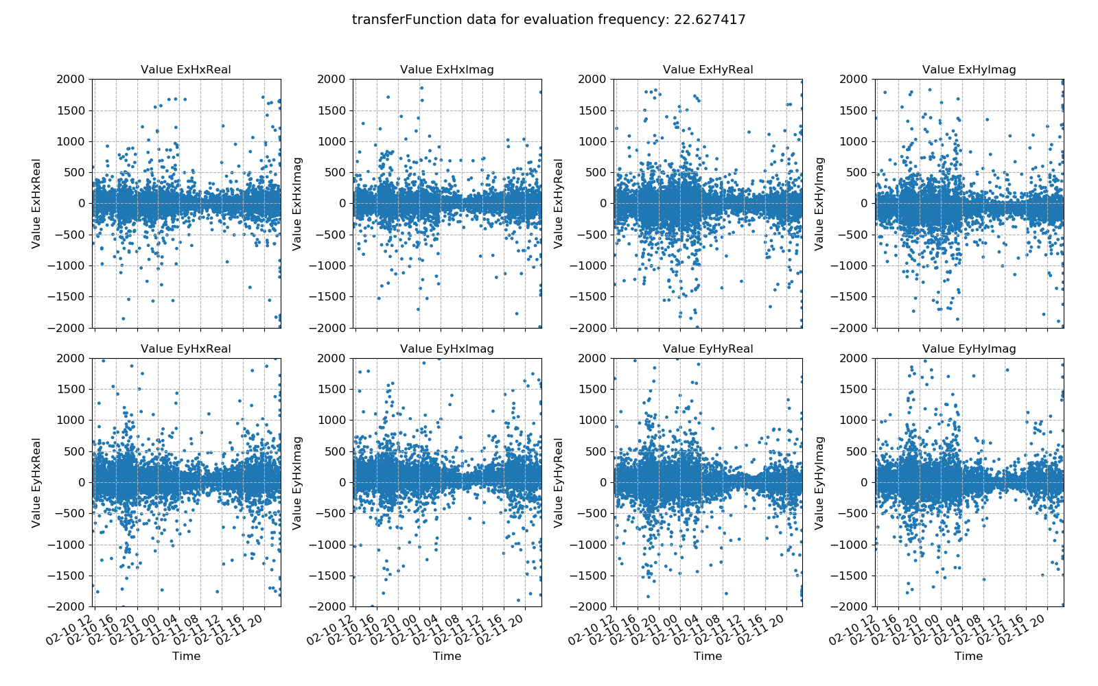
Decimation Level = 0: 32.00000000, 22.62741700, 16.00000000, 11.31370850, 8.00000000 Decimation Level = 1: 5.65685425, 4.00000000, 2.82842712, 2.00000000, 1.41421356 Decimation Level = 2: 1.00000000, 0.70710678, 0.50000000, 0.35355339, 0.25000000 Decimation Level = 3: 0.17677670, 0.12500000, 0.08838835, 0.06250000, 0.04419417 Decimation Level = 4: 0.03125000, 0.02209709, 0.01562500, 0.01104854, 0.00781250 Decimation Level = 5: 0.00552427, 0.00390625, 0.00276214, 0.00195312, 0.00138107 Decimation Level = 6: 0.00097656, 0.00069053, 0.00048828, 0.00034527, 0.00024414 Decimation Level = 7: 0.00017263, 0.00012207, 0.00008632, 0.00006104, 0.00004316Decimation level numbering starts from 0 (and with 8 decimation levels, extends to 7). Evaluation frequency numbering begins from 0 (and with 5 evaluation frequencies per decimation level, extends to 4).
The decimation and evaluation frequency indices can be best demonstrated using a few of examples:
Evaluation frequency 32 Hz, decimation level = 0, evaluation frequency index = 0
Evaluation frequency 1 Hz, decimation level = 2, evaluation frequency index = 0
Evaluation frequency 0.35355339 Hz, decimation level = 2, evaluation frequency index = 3
The main motivation behind this is the difficulty in manually specifying evaluation frequencies such as 0.35355339 Hz.
Below are examples of plotting site and sampling frequency wide statistics for different evaluation frequencies and decimation levels.
113 114 115 116 117 118 119 120 121 122 123 124 125 126 127 128 129 130 131 132 133 134 135 136 137 138 139 | # more examples
# change the evaluation frequency
fig = viewStatistic(
projData,
"site1",
128,
"transferFunction",
ylim=[-2000, 2000],
eFreqI=1,
save=False,
show=False,
)
fig.savefig(imagePath / "usingStats_projstat_transfunction_view_efreq")
# change the decimation level
fig = viewStatistic(
projData,
"site1",
128,
"transferFunction",
ylim=[-2000, 2000],
declevel=1,
eFreqI=0,
save=False,
show=False,
)
fig.savefig(imagePath / "usingStats_projstat_transfunction_view_declevel")
|
Transfer function data plotted for all time series measurements of a given sampling frequency in a site using the viewStatistic(). Here, evaluation frequency 22.627417 Hz is plotted (decimation level = 0, evaluation frequency index = 1).
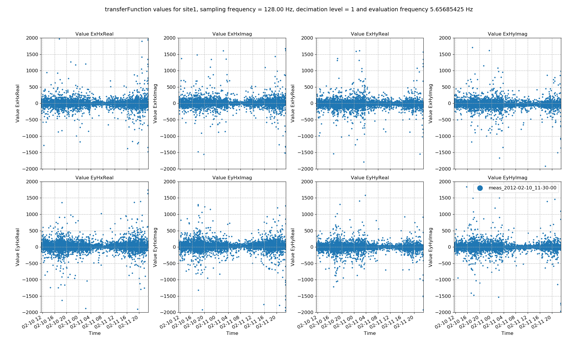
Transfer function data plotted for all time series measurements of a given sampling frequency in a site using the viewStatistic(). Here, evaluation frequency 5.65685425 Hz is plotted (decimation level = 1, evaluation frequency index = 0).
Up until now, statistics have been used to investigate the variance of the time series data. However, they can be used to select which time windows to process. To find out how to use them to select and remove time windows, continue to the Masks section.
Complete example script
For the purposes of clarity, the complete example script is provided below.
1 2 3 4 5 6 7 8 9 10 11 12 13 14 15 16 17 18 19 20 21 22 23 24 25 26 27 28 29 30 31 32 33 34 35 36 37 38 39 40 41 42 43 44 45 46 47 48 49 50 51 52 53 54 55 56 57 58 59 60 61 62 63 64 65 66 67 68 69 70 71 72 73 74 75 76 77 78 79 80 81 82 83 84 85 86 87 88 89 90 91 92 93 94 95 96 97 98 99 100 101 102 103 104 105 106 107 108 109 110 111 112 113 114 115 116 117 118 119 120 121 122 123 124 125 126 127 128 129 130 131 132 133 134 135 136 137 138 139 | from datapaths import projectPath, imagePath
from resistics.project.io import loadProject
# need the project path for loading
projData = loadProject(projectPath)
# get default statistic names
from resistics.statistics.utils import getStatNames

stats, remotestats = getStatNames()
# calculate statistics
from resistics.project.statistics import calculateStatistics

calculateStatistics(projData, stats=stats)
# calculate statistics for a different spectra directory
# load the project with the tutorial configuration file
projData = loadProject(projectPath, configFile="tutorialConfig.ini")
projData.printInfo()
calculateStatistics(projData, stats=stats)
# to get statistic data, we need the site, the measurement and the statistic we want
from resistics.project.statistics import getStatisticData

# coherence statistic data
statData = getStatisticData(
    projData, "site1", "meas_2012-02-10_11-30-00", "coherence", declevel=0
)
# view statistic value over time
fig = statData.view(0)
fig.savefig(imagePath / "usingStats_statistic_coherence_view")
# view statistic histogram
fig = statData.histogram(0)
fig.savefig(imagePath / "usingStats_statistic_coherence_histogram")
# view statistic crossplot
fig = statData.crossplot(0, crossplots=[["cohExHy", "cohEyHx"], ["cohExHx", "cohEyHy"]])
fig.savefig(imagePath / "usingStats_statistic_coherence_crossplot")
# view statistic density plot
fig = statData.densityplot(
    0,
    crossplots=[["cohExHy", "cohEyHx"], ["cohExHx", "cohEyHy"]],
    xlim=[0, 1],
    ylim=[0, 1],
)
fig.savefig(imagePath / "usingStats_statistic_coherence_densityplot")
# transfer function statistic data
statData = getStatisticData(
    projData, "site1", "meas_2012-02-10_11-30-00", "transferFunction", declevel=0
)
# view statistic value over time
fig = statData.view(0, ylim=[-2000, 2000])
fig.savefig(imagePath / "usingStats_statistic_transferfunction_view")
# view statistic histogram
fig = statData.histogram(0, xlim=[-500, 500])
fig.savefig(imagePath / "usingStats_statistic_transferfunction_histogram")
# view statistic crossplot
fig = statData.crossplot(
    0,
    crossplots=[
        ["ExHxReal", "ExHxImag"],
        ["ExHyReal", "ExHyImag"],
        ["EyHxReal", "EyHxImag"],
        ["EyHyReal", "EyHyImag"],
    ],
    xlim=[-2500, 2500],
    ylim=[-2500, 2500],
)
fig.savefig(imagePath / "usingStats_statistic_transferfunction_crossplot")
# view statistic densityplot
fig = statData.densityplot(
    0,
    crossplots=[
        ["ExHxReal", "ExHxImag"],
        ["ExHyReal", "ExHyImag"],
        ["EyHxReal", "EyHxImag"],
        ["EyHyReal", "EyHyImag"],
    ],
    xlim=[-60, 60],
    ylim=[-60, 60],
)
fig.savefig(imagePath / "usingStats_statistic_transferfunction_densityplot")
# look at the next evaluation frequency
fig = statData.view(1, ylim=[-2000, 2000])
fig.savefig(imagePath / "usingStats_statistic_transferfunction_view_eval1")
# plot statistic values in time for all data of a specified sampling frequency in a site
from resistics.project.statistics import viewStatistic

# statistic in time
fig = viewStatistic(
    projData,
    "site1",
    128,
    "transferFunction",
    ylim=[-2000, 2000],
    save=False,
    show=False,
)
fig.savefig(imagePath / "usingStats_projstat_transfunction_view")
# plot statistic histogram for all data of a specified sampling frequency in a site
from resistics.project.statistics import viewStatisticHistogram

# statistic histogram
fig = viewStatisticHistogram(
    projData, "site1", 128, "transferFunction", xlim=[-500, 500], save=False, show=False
)
fig.savefig(imagePath / "usingStats_projstat_transfunction_hist")
# more examples
# change the evaluation frequency
fig = viewStatistic(
    projData,
    "site1",
    128,
    "transferFunction",
    ylim=[-2000, 2000],
    eFreqI=1,
    save=False,
    show=False,
)
fig.savefig(imagePath / "usingStats_projstat_transfunction_view_efreq")

# change the decimation level
fig = viewStatistic(
    projData,
    "site1",
    128,
    "transferFunction",
    ylim=[-2000, 2000],
    declevel=1,
    eFreqI=0,
    save=False,
    show=False,
)
fig.savefig(imagePath / "usingStats_projstat_transfunction_view_declevel")
|