Viewing spectra
Spectra data is stored in the following locations.
exampleProject
├── calData
├── timeData
│   └── site1
|       |── dataFolder1
│       |── dataFolder2
|       |──     .
|       |──     .
|       |──     .
|       └── dataFolderN
├── specData
│   └── site1
|       |── dataFolder1
|       |   └── spectra
│       |── dataFolder2
|       |   └── spectra
|       |──     .
|       |──     .
|       |──     .
|       └── dataFolderN
|           └── spectra
├── statData
├── maskData
├── transFuncData
├── images
└── mtProj.prj
Each spectra file that is calculated is written out with a set of comments. The comment file is a text file that can be opened in any text editor and records the various parameters used when calculating out spectra. An example is given below.
1 2 3 4 5 6 7 8 9 10 11 12 13 14 15 16 17 18 19 20 21 22 23 24 25 26 27 28 29 30 31 32 33 34 35 36 | Unscaled data 2012-02-10 11:30:00 to 2012-02-11 23:03:43.992188 read in from measurement E:\magnetotellurics\code\resisticsdata\tutorial\tutorialProject\timeData\site1\meas_2012-02-10_11-30-00, samples 0 to 16387071
Sampling frequency 128.0
Scaling channel Ex with scalar -0.000112591 to give mV
Dividing channel Ex by electrode distance 0.08 km to give mV/km
Scaling channel Ey with scalar -0.000112512 to give mV
Dividing channel Ey by electrode distance 0.091 km to give mV/km
Scaling channel Hx with scalar -0.00360174 to give mV
Scaling channel Hy with scalar -0.00360038 to give mV
Scaling channel Hz with scalar -0.0036007 to give mV
Remove zeros: False, remove nans: False, remove average: True
---------------------------------------------------
Calculating project spectra
Using default configuration
Channel Ex not calibrated
Channel Ey not calibrated
Channel Hx calibrated with calibration data from file E:\magnetotellurics\code\resisticsdata\tutorial\tutorialProject\calData\Hx_MFS06365.TXT
Channel Hy calibrated with calibration data from file E:\magnetotellurics\code\resisticsdata\tutorial\tutorialProject\calData\Hy_MFS06357.TXT
Channel Hz calibrated with calibration data from file E:\magnetotellurics\code\resisticsdata\tutorial\tutorialProject\calData\Hz_MFS06307.TXT
Decimating with 7 levels and 7 frequencies per level
Evaluation frequencies for this level 32.0, 22.62741699796952, 16.0, 11.31370849898476, 8.0, 5.65685424949238, 4.0
Windowing with window size 512 samples and overlap 128 samples
Time data decimated from 128.0 Hz to 16.0 Hz, new start time 2012-02-10 11:30:00, new end time 2012-02-11 23:03:43.937500
Evaluation frequencies for this level 2.82842712474619, 2.0, 1.414213562373095, 1.0, 0.7071067811865475, 0.5, 0.35355339059327373
Windowing with window size 512 samples and overlap 128 samples
Time data decimated from 16.0 Hz to 2.0 Hz, new start time 2012-02-10 11:30:00, new end time 2012-02-11 23:03:43.500000
Evaluation frequencies for this level 0.25, 0.17677669529663687, 0.125, 0.08838834764831843, 0.0625, 0.044194173824159216, 0.03125
Windowing with window size 512 samples and overlap 128 samples
Time data decimated from 2.0 Hz to 0.25 Hz, new start time 2012-02-10 11:30:00, new end time 2012-02-11 23:03:40
Time data decimated from 0.25 Hz to 0.125 Hz, new start time 2012-02-10 11:30:00, new end time 2012-02-11 23:03:36
Evaluation frequencies for this level 0.022097086912079608, 0.015625, 0.011048543456039804, 0.0078125, 0.005524271728019902, 0.00390625, 0.002762135864009951
Windowing with window size 512 samples and overlap 128 samples
Time data decimated from 0.125 Hz to 0.015625 Hz, new start time 2012-02-10 11:30:00, new end time 2012-02-11 23:03:20
Evaluation frequencies for this level 0.001953125, 0.0013810679320049755, 0.0009765625, 0.0006905339660024878, 0.00048828125, 0.0003452669830012439, 0.000244140625
Windowing with window size 512 samples and overlap 128 samples
Spectra data written out to E:\magnetotellurics\code\resisticsdata\tutorial\tutorialProject\specData\site1\meas_2012-02-10_11-30-00\spectra on 2019-10-05 19:17:48.174074 using resistics 0.0.6.dev2
---------------------------------------------------
|
There are a few methods in the project spectra module that can be used to visualise spectra. These are:
View raw spectra data for time windows
View spectra sections - an image of spectras calculated over the period of recording
View spectra periodograms
To begin looking at spectra, load the project in the standard way.
1 2 3 4 5 | from datapaths import projectPath, imagePath
from resistics.project.io import loadProject
# load the project
projData = loadProject(projectPath)
|
The fourier spectra can be viewed using the viewSpectra() method, which takes a site and measurement as arguments.
7 8 9 10 11 | # view the spectra at 128 Hz
from resistics.project.spectra import viewSpectra
fig = viewSpectra(projData, "site1", "meas_2012-02-10_11-30-00", show=False, save=False)
fig.savefig(imagePath / "viewSpec_projspec_128_view")
|
This gives the following output:
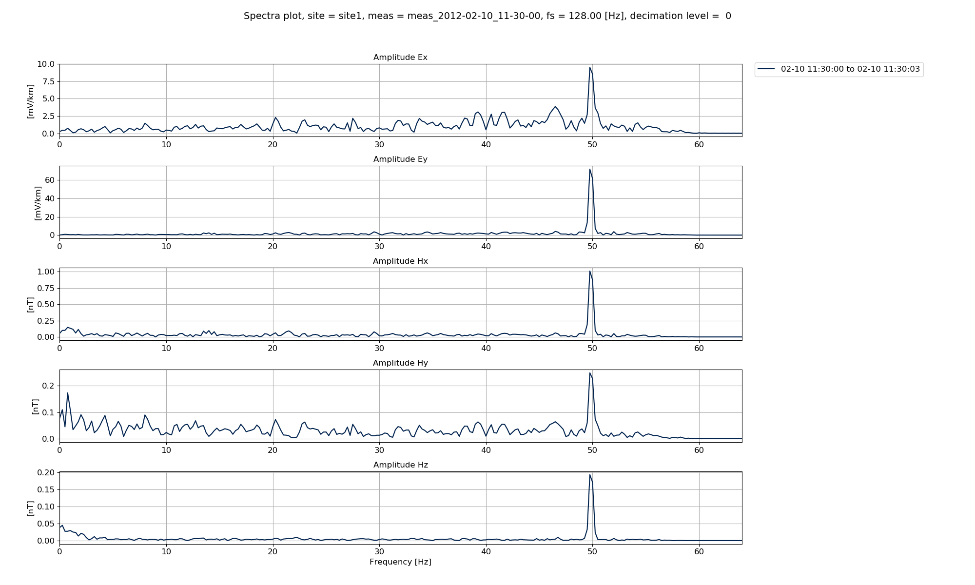
Plot of the first time window spectrum
Plotting options can be defined using the plotoptions keyword for viewSpectra(). This needs to be a dictionary defining layout options (limits etc). There are some built-in plot options for different types of plots. In the below example, plotOptionsSpec() returns a dictionary of standard plot options for spectra. Further, getPaperFonts() returns a dictionary of font sizes to use for the plot targetted at papers.
13 14 15 16 17 | # setting the plot options
from resistics.common.plot import plotOptionsSpec, getPaperFonts
plotOptions = plotOptionsSpec(plotfonts=getPaperFonts())
print(plotOptions)
|
The plot options dictionary looks like this:
{'figsize': (20, 12), 'plotfonts': {'suptitle': 18, 'title': 17, 'axisLabel': 16, 'axisTicks': 15, 'legend': 15}, 'block': True, 'amplim': []}
Now plotting the spectra again with the new plot options gives the same plot but with bigger font sizes which might be useful for an academic paper.
19 20 21 22 23 24 25 26 27 28 | # view the spectra at 128 Hz
fig = viewSpectra(
projData,
"site1",
"meas_2012-02-10_11-30-00",
plotoptions=plotOptions,
show=False,
save=False,
)
fig.savefig(imagePath / "viewSpec_projspec_128_view_plotoptions")
|
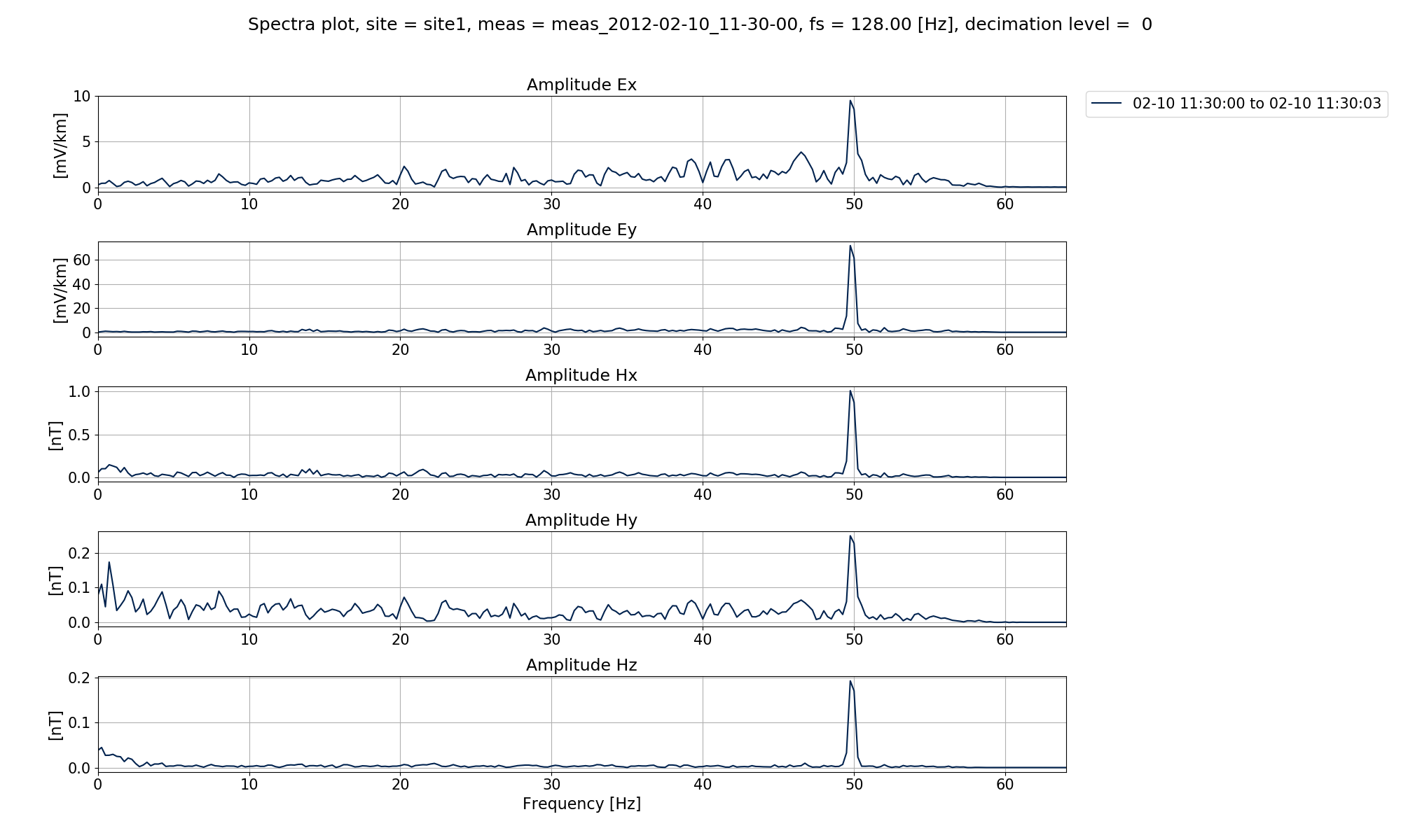
Plot of the first time window spectrum using a different set of plot options
Currently, this is only plotting the spectrum of the first time window. To explore variation, more than a single time window can be plotted. This is achieved using the plotwindow keyword. The plotwindow keyword can be:
An integer which is the local index of the time window (local index means referenced to the start time of the time series)
“all”, which will plot 20 windows across the duration of the whole measurement
A dictionary with a start and stop, i.e. {start: 30, stop:40}, which will then define the range 30, 31, 32, 33, 34, 35, 36, 37, 38, 39 and 40
In the below example, plotwindow = “all” which means that 20 windows across the time series measurement will be plotted.
30 31 32 33 34 35 36 37 38 39 40 41 | # view the spectra at 128 Hz for more than a single window
fig = viewSpectra(
projData,
"site1",
"meas_2012-02-10_11-30-00",
chans=["Ex", "Hy"],
plotwindow="all",
plotoptions=plotOptions,
show=False,
save=False,
)
fig.savefig(imagePath / "viewSpec_projspec_128_view_plotall_chans")
|
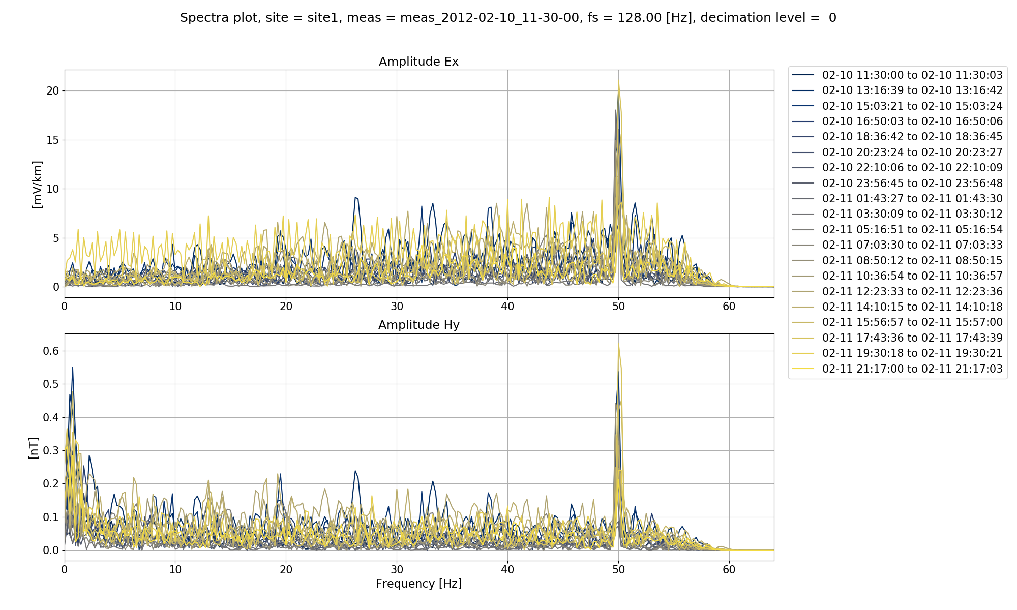
Plot of multiple window spectra
Another useful way to inspect the variation of spectra across the time series measurement is to plot a spectra section using the viewSpectraSection() method of the project spectra module. This is a 2-D image of the spectra with time across the x-axis and frequency across the y-axis with colour representing the amplitude. An example of plotting a spectra section and the image is shown below.
41 42 43 44 45 46 47 48 49 50 51 52 | # spectra sections
from resistics.project.spectra import viewSpectraSection
fig = viewSpectraSection(
projData,
"site1",
"meas_2012-02-10_11-30-00",
plotoptions=plotOptions,
show=False,
save=False,
)
fig.savefig(imagePath / "viewSpec_projspec_128_section")
|
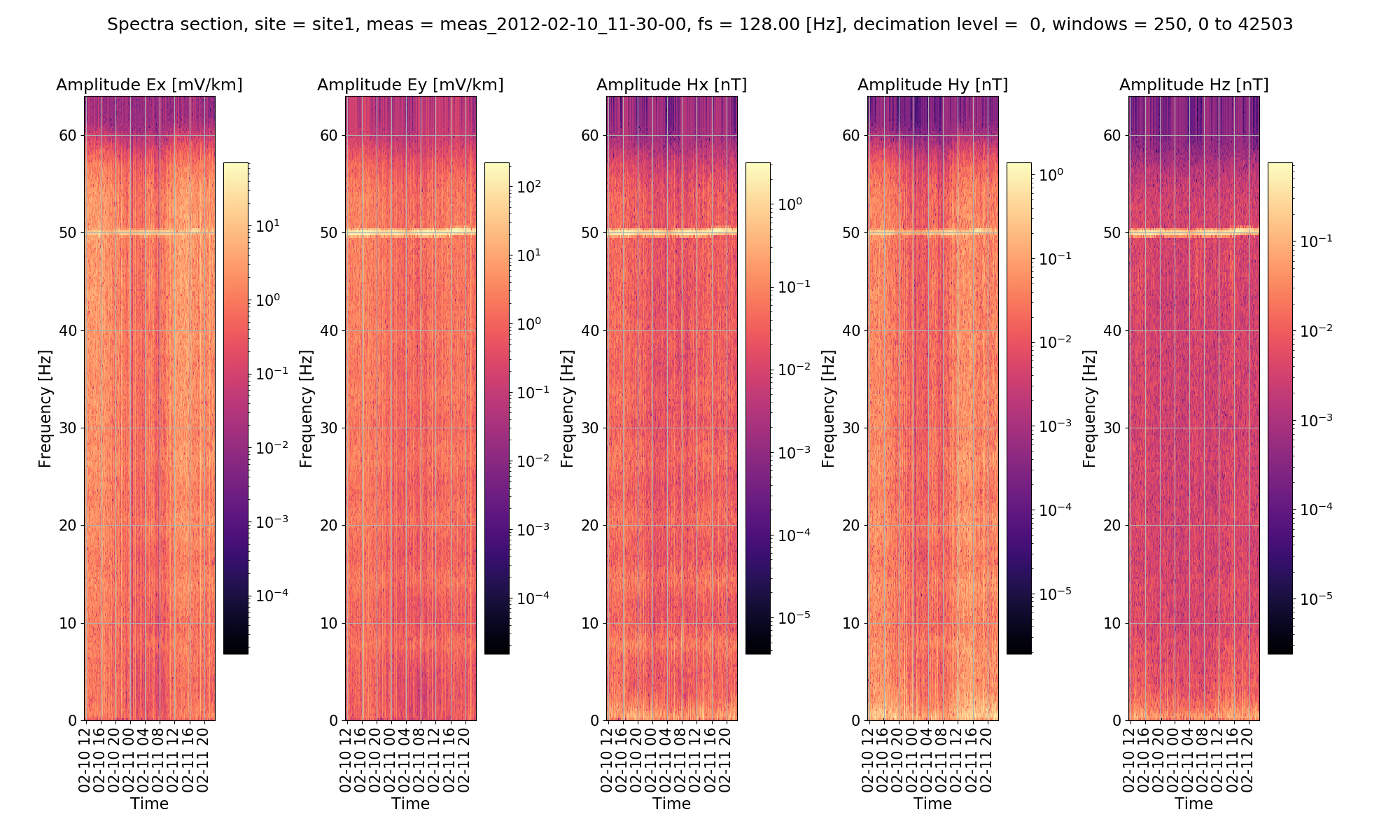
Plot of a spectra section for 128Hz sampling frequency data
Spectra sections plot 250 window spectra across the duration of the time series measurement.
To understand the dominant frequencies in a time series measurement, it can be useful to perform spectral stacking. This can be achieved using the viewSpectraStack() method of the project spectra module. Spectra stacking will averages the spectra amplitudes across multiple windows.
56 57 58 59 60 61 62 63 64 65 66 67 68 | # spectra stack
from resistics.project.spectra import viewSpectraStack
fig = viewSpectraStack(
projData,
"site1",
"meas_2012-02-10_11-30-00",
coherences=[["Ex", "Hy"], ["Ey", "Hx"]],
plotoptions=plotOptions,
show=False,
save=False,
)
fig.savefig(imagePath / "viewSpec_projspec_128_stack")
|
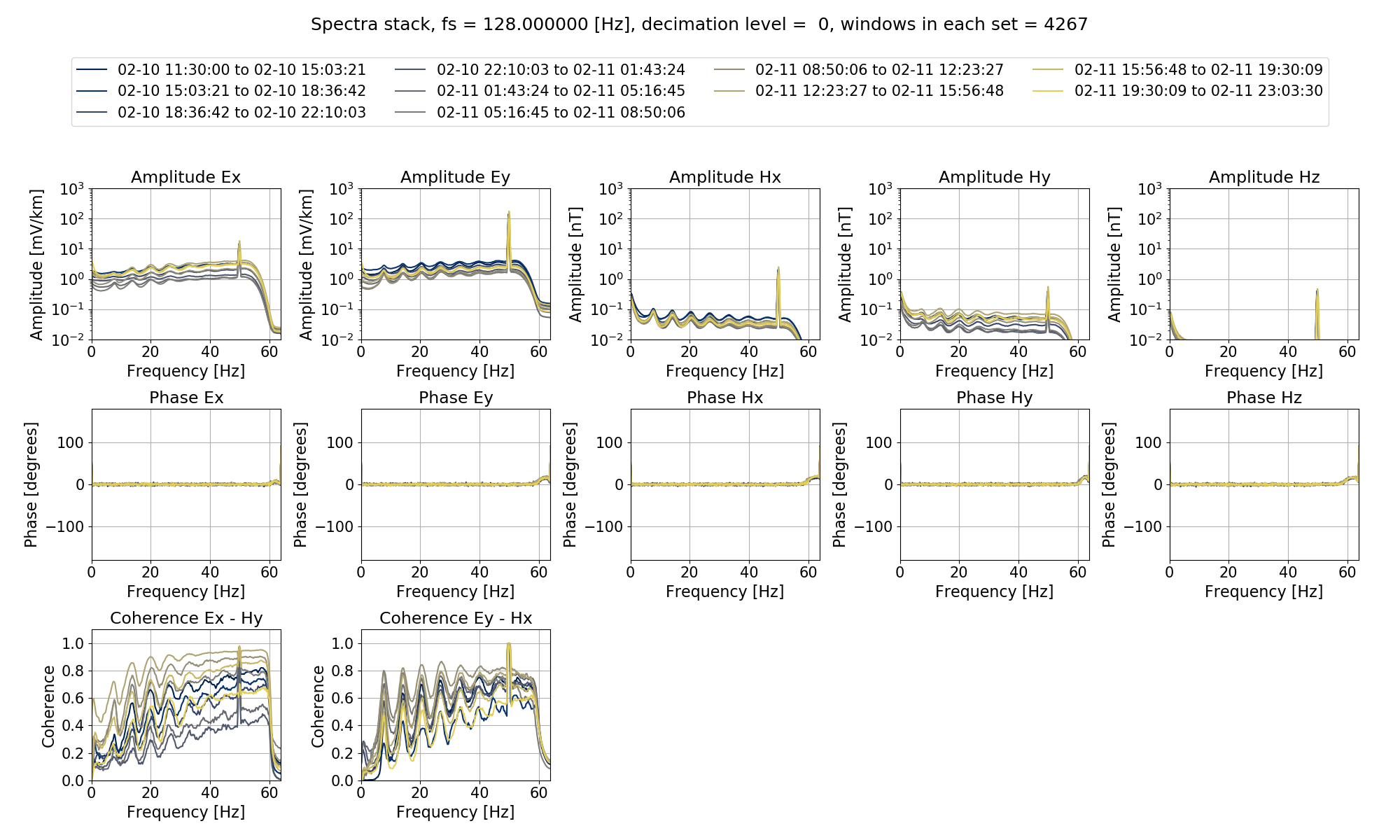
Plot of a spectra stacking for 128Hz sampling frequency data
Adding the coherences keyword also stacks the coherences. The number of stacks to perform across the duration of the time series measurement can be controlled using the numstacks keyword. For more information, see the documentation for viewSpectraStack().
The above were demonstrated on data sampled at 128Hz sampling rate but can be easily repeated for the 4096Hz data of the tutorial project.
70 71 72 73 74 75 76 77 78 79 80 81 82 83 84 85 86 87 88 89 90 91 92 93 94 95 96 97 98 99 100 101 | # view the spectra at 4096 Hz
fig = viewSpectra(
projData,
"site1",
"meas_2012-02-10_11-05-00",
plotwindow="all",
plotoptions=plotOptions,
show=False,
save=False,
)
fig.savefig(imagePath / "viewSpec_projspec_4096_view_plotall")
fig = viewSpectraSection(
projData,
"site1",
"meas_2012-02-10_11-05-00",
plotoptions=plotOptions,
show=False,
save=False,
)
fig.savefig(imagePath / "viewSpec_projspec_4096_view_section")
fig = viewSpectraStack(
projData,
"site1",
"meas_2012-02-10_11-05-00",
coherences=[["Ex", "Hy"], ["Ey", "Hx"]],
plotoptions=plotOptions,
show=False,
save=False,
)
fig.savefig(imagePath / "viewSpec_projspec_4096_view_stack_coherences")
|
The resultant plots are:
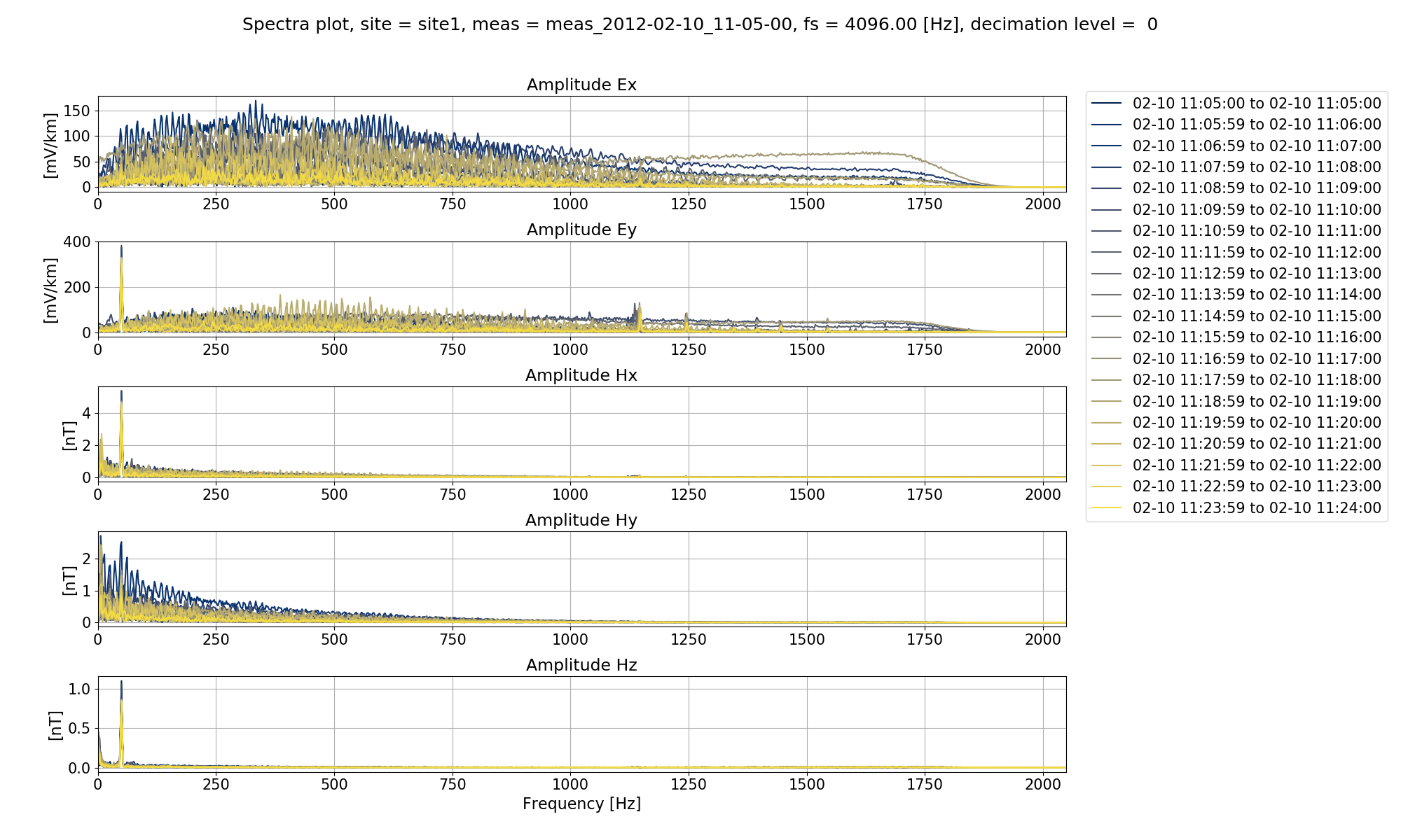
Plot of a spectra for 20 windows across the 4096Hz measurement
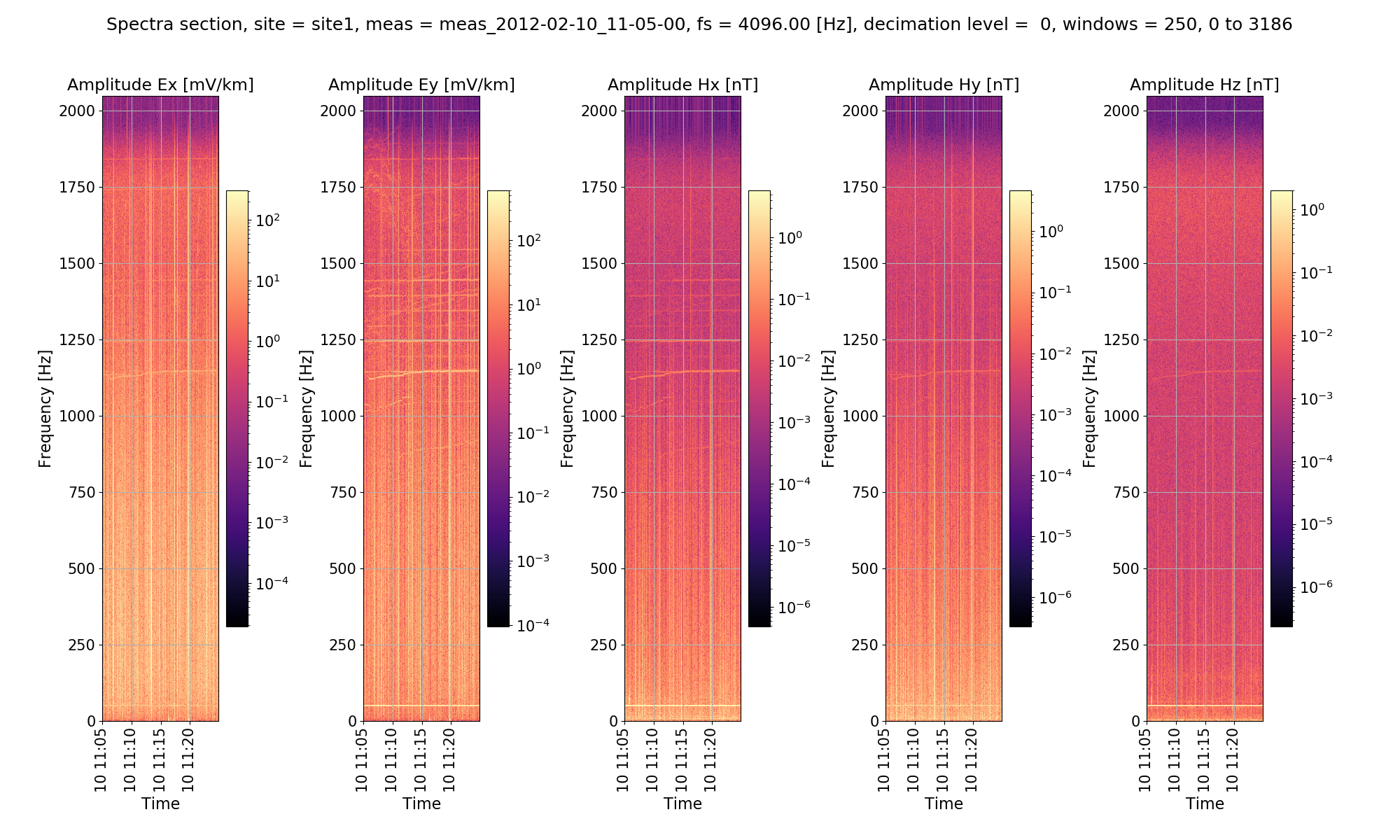
Plot of spectra section for the 4096Hz measurement
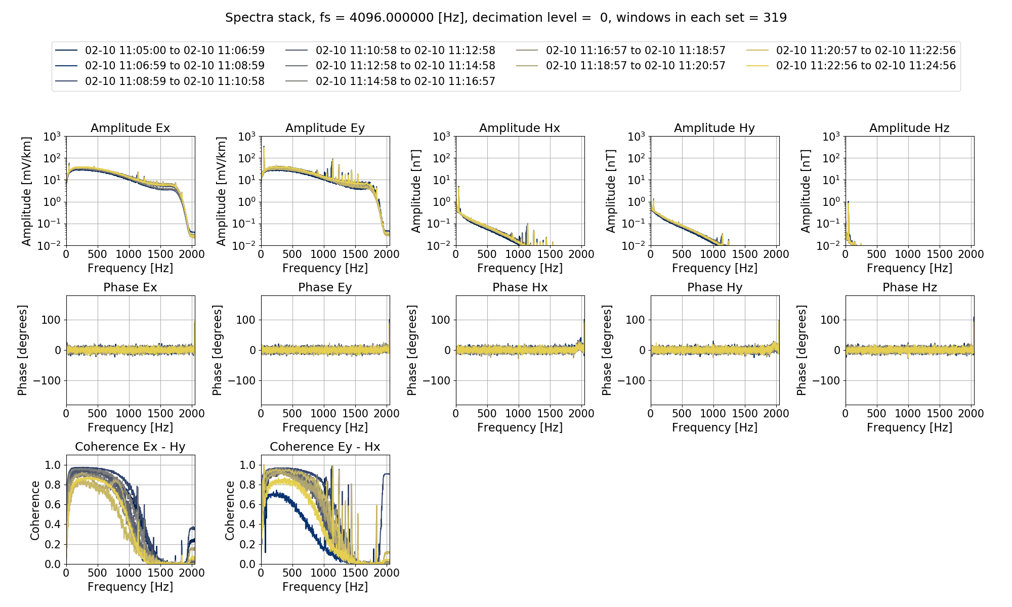
Plot of spectra stack for the 4096Hz measurement
All the above are a means to understand the dominant frequencies in the time series data. Ideally, the Schumann resonances should be visible, as they are in the 128Hz data. Other common features are powerline noise - the exact frequency of this is dependent on geographic location, but often 50Hz - and trainline noise around 16.6Hz.
Complete example script
For the purposes of clarity, the complete example script is provided below.
1 2 3 4 5 6 7 8 9 10 11 12 13 14 15 16 17 18 19 20 21 22 23 24 25 26 27 28 29 30 31 32 33 34 35 36 37 38 39 40 41 42 43 44 45 46 47 48 49 50 51 52 53 54 55 56 57 58 59 60 61 62 63 64 65 66 67 68 69 70 71 72 73 74 75 76 77 78 79 80 81 82 83 84 85 86 87 88 89 90 91 92 93 94 95 96 97 98 99 100 101 | from datapaths import projectPath, imagePath
from resistics.project.io import loadProject
# load the project
projData = loadProject(projectPath)
# view the spectra at 128 Hz
from resistics.project.spectra import viewSpectra

fig = viewSpectra(projData, "site1", "meas_2012-02-10_11-30-00", show=False, save=False)
fig.savefig(imagePath / "viewSpec_projspec_128_view")
# setting the plot options
from resistics.common.plot import plotOptionsSpec, getPaperFonts

plotOptions = plotOptionsSpec(plotfonts=getPaperFonts())
print(plotOptions)
# view the spectra at 128 Hz
fig = viewSpectra(
    projData,
    "site1",
    "meas_2012-02-10_11-30-00",
    plotoptions=plotOptions,
    show=False,
    save=False,
)
fig.savefig(imagePath / "viewSpec_projspec_128_view_plotoptions")
# view the spectra at 128 Hz for more than a single window
fig = viewSpectra(
    projData,
    "site1",
    "meas_2012-02-10_11-30-00",
    chans=["Ex", "Hy"],
    plotwindow="all",
    plotoptions=plotOptions,
    show=False,
    save=False,
)
fig.savefig(imagePath / "viewSpec_projspec_128_view_plotall_chans")
# spectra sections
from resistics.project.spectra import viewSpectraSection

fig = viewSpectraSection(
    projData,
    "site1",
    "meas_2012-02-10_11-30-00",
    plotoptions=plotOptions,
    show=False,
    save=False,
)
fig.savefig(imagePath / "viewSpec_projspec_128_section")
# spectra stack
from resistics.project.spectra import viewSpectraStack

fig = viewSpectraStack(
    projData,
    "site1",
    "meas_2012-02-10_11-30-00",
    coherences=[["Ex", "Hy"], ["Ey", "Hx"]],
    plotoptions=plotOptions,
    show=False,
    save=False,
)
fig.savefig(imagePath / "viewSpec_projspec_128_stack")
# view the spectra at 4096 Hz
fig = viewSpectra(
    projData,
    "site1",
    "meas_2012-02-10_11-05-00",
    plotwindow="all",
    plotoptions=plotOptions,
    show=False,
    save=False,
)
fig.savefig(imagePath / "viewSpec_projspec_4096_view_plotall")

fig = viewSpectraSection(
    projData,
    "site1",
    "meas_2012-02-10_11-05-00",
    plotoptions=plotOptions,
    show=False,
    save=False,
)
fig.savefig(imagePath / "viewSpec_projspec_4096_view_section")

fig = viewSpectraStack(
    projData,
    "site1",
    "meas_2012-02-10_11-05-00",
    coherences=[["Ex", "Hy"], ["Ey", "Hx"]],
    plotoptions=plotOptions,
    show=False,
    save=False,
)
fig.savefig(imagePath / "viewSpec_projspec_4096_view_stack_coherences")
|