Viewing timeseries data
After time data files are in place, they can be visualised. Begin by loading the project and then using the methods in the project time module.
1 2 3 4 5 6 7 8 9 10 11 12 13 14 | from datapaths import projectPath, imagePath
from resistics.project.io import loadProject
# load the project
projData = loadProject(projectPath)
# load the viewing method
from resistics.project.time import viewTime
# view data between certain date range
fig = viewTime(
projData, "2012-02-11 01:00:00", "2012-02-11 01:10:00", show=False, save=False
)
fig.savefig(imagePath / "viewTime_projtime_view")
|
This yields the below plot:
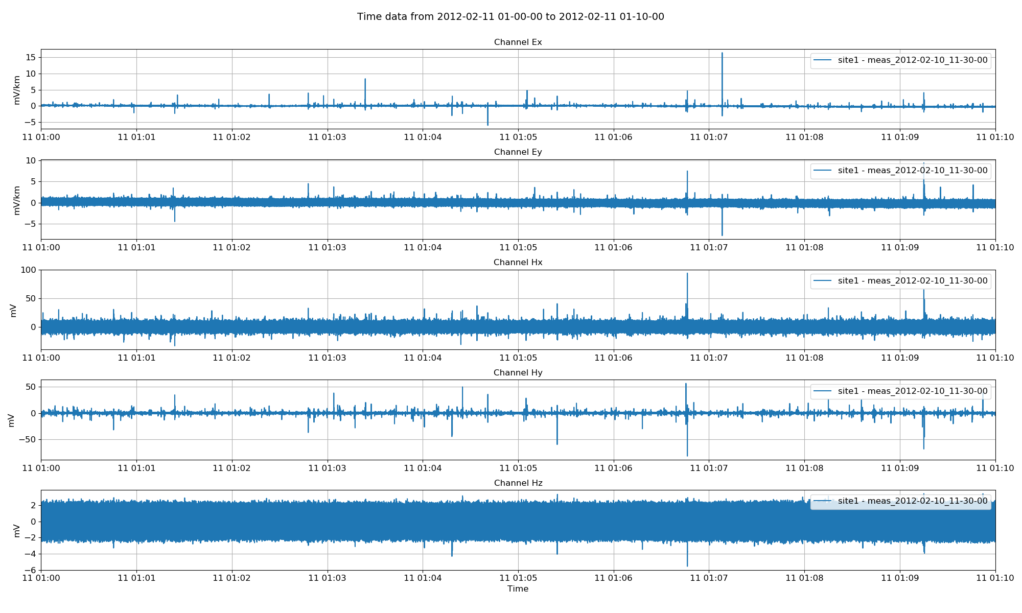
Project time data
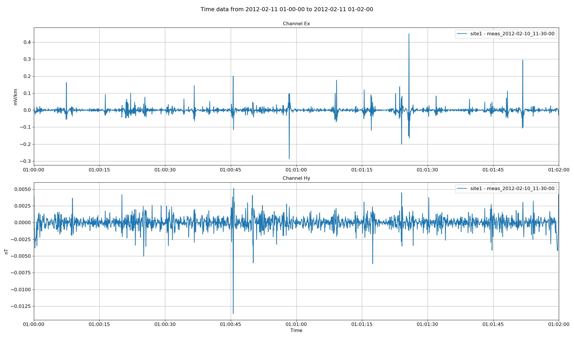
By default, channels Ex, Ey, Hx, Hy, Hz are all plotted. However, the channels to plot can be explicitly defined. Further, all sites in the project with time data in this range will be plotted. Sites to plot can be explicitly defined as a list of sites.
16 17 18 19 20 21 22 23 24 25 26 | # explicitly define sites and channels to plot
fig = viewTime(
projData,
"2012-02-11 01:00:00",
"2012-02-11 01:02:00",
sites=["site1"],
chans=["Ex", "Hy"],
show=False,
save=False,
)
fig.savefig(imagePath / "viewTime_projtime_view_chans")
|
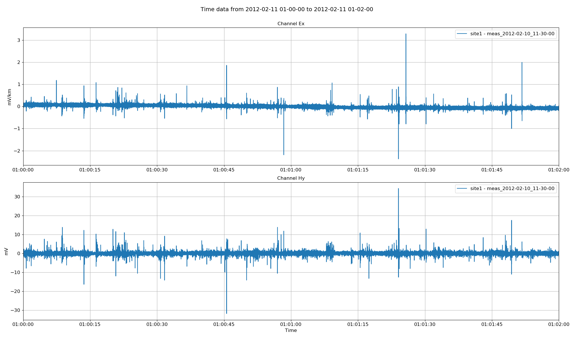
Project time data with sites and channels restricted
There are a number of pre-processing options that can be optionally applied to the time data. If calibration files for magnetic channels are available and appropriately placed in the project calData directory, the calibration option can be applied.
28 29 30 31 32 33 34 35 36 37 38 39 | # calibrate magnetic channels
fig = viewTime(
projData,
"2012-02-11 01:00:00",
"2012-02-11 01:02:00",
sites=["site1"],
chans=["Ex", "Hy"],
calibrate=True,
show=False,
save=False,
)
fig.savefig(imagePath / "viewTime_projtime_view_calibrate")
|
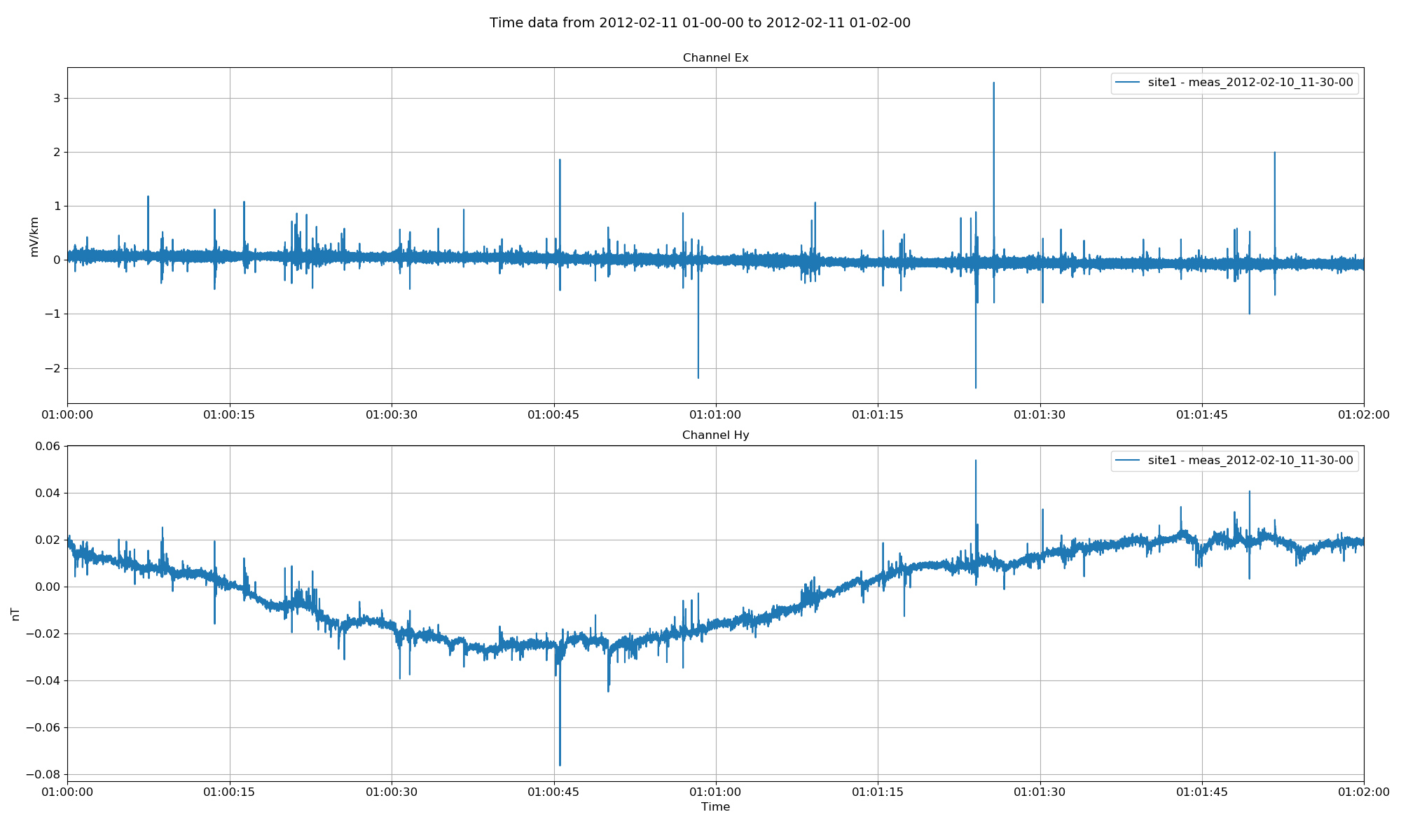
Project time data with magnetic fields calibrated
Low pass filters can be applied to the data as shown below:
41 42 43 44 45 46 47 48 49 50 51 52 53 | # low pass filter
fig = viewTime(
projData,
"2012-02-11 01:00:00",
"2012-02-11 01:02:00",
sites=["site1"],
chans=["Ex", "Hy"],
calibrate=True,
filter={"lpfilt": 0.5},
show=False,
save=False,
)
fig.savefig(imagePath / "viewTime_projtime_view_calibrate_lpfilt")
|
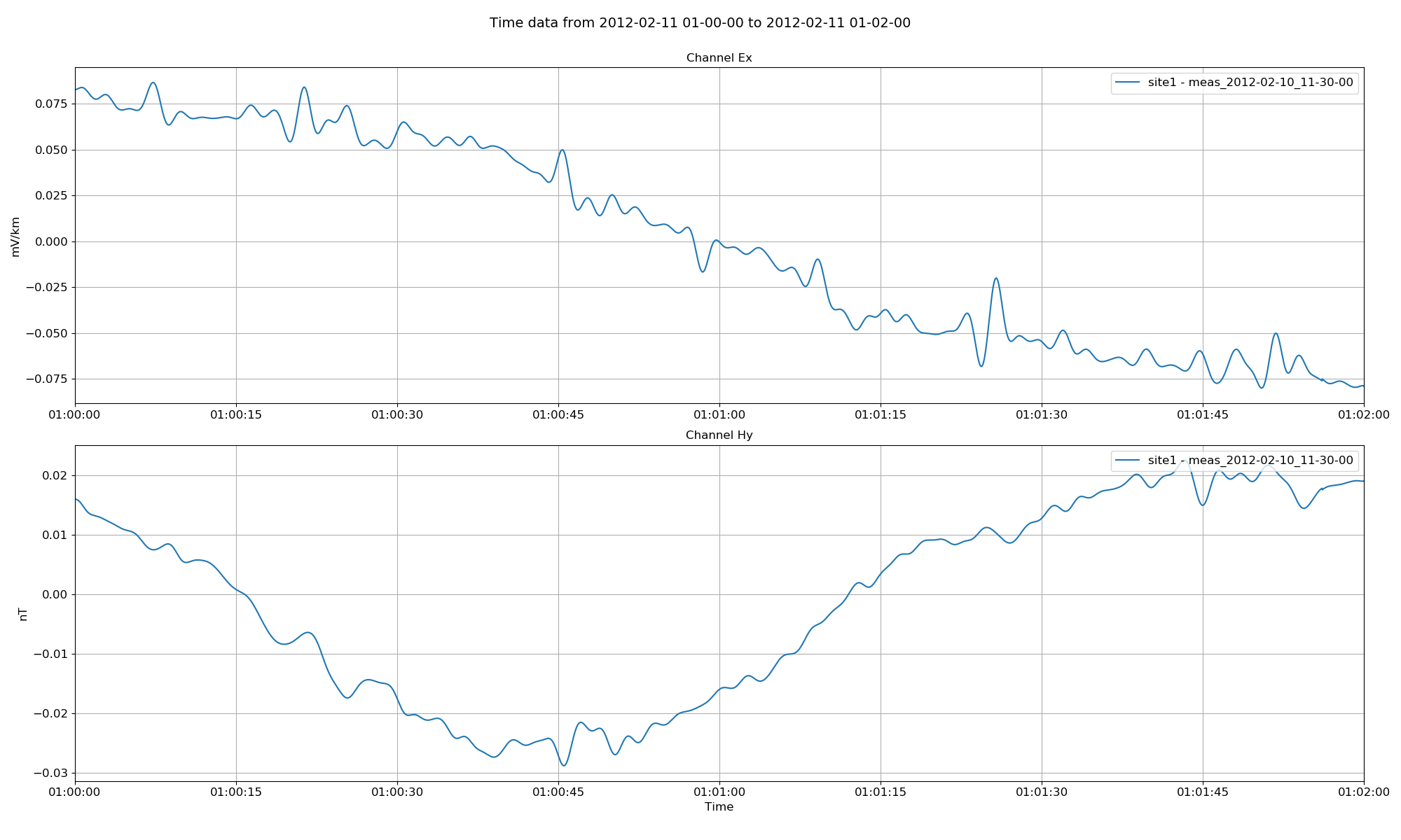
Project time data with magnetic fields calibrated and a low pass filter applied
High pass, band pass and notch filters can also be applied to the data in a similar fashion.
55 56 57 58 59 60 61 62 63 64 65 66 67 68 69 70 71 72 73 74 75 76 77 78 79 80 81 82 83 84 85 86 87 88 89 90 91 92 93 94 95 | # high pass filter
fig = viewTime(
projData,
"2012-02-11 01:00:00",
"2012-02-11 01:02:00",
sites=["site1"],
chans=["Ex", "Hy"],
calibrate=True,
filter={"hpfilt": 10},
show=False,
save=False,
)
fig.savefig(imagePath / "viewTime_projtime_view_calibrate_hpfilt")
# band pass filter
fig = viewTime(
projData,
"2012-02-11 01:00:00",
"2012-02-11 01:02:00",
sites=["site1"],
chans=["Ex", "Hy"],
calibrate=True,
filter={"bpfilt": [1, 10]},
show=False,
save=False,
)
fig.savefig(imagePath / "viewTime_projtime_view_calibrate_bpfilt")
# notch
fig = viewTime(
projData,
"2012-02-11 01:00:00",
"2012-02-11 01:02:00",
sites=["site1"],
chans=["Ex", "Hy"],
calibrate=True,
notch=[16.6667, 50],
show=False,
save=False,
)
fig.savefig(imagePath / "viewTime_projtime_view_calibrate_notch")
|
The channels can be individually normalised by using the normalise option. The normalisation factor here is calculated using the numpy.linalg.norm method.
97 98 99 100 101 102 103 104 105 106 107 108 109 | # normalise
fig = viewTime(
projData,
"2012-02-11 01:00:00",
"2012-02-11 01:02:00",
sites=["site1"],
chans=["Ex", "Hy"],
calibrate=True,
normalise=True,
show=False,
save=False,
)
fig.savefig(imagePath / "viewTime_projtime_view_calibrate_normalise")
|
Resistics can automatically save plots as images in the project images directory. When batching, it can often be useful to not show the plots (which tend to block the progress of the code) but rather save the plot without showing it. This can be achieved in the following way:
111 112 113 114 115 116 117 118 119 120 121 122 123 | # save with band pass filter
fig = viewTime(
projData,
"2012-02-11 01:00:00",
"2012-02-11 01:02:00",
sites=["site1"],
chans=["Ex", "Hy"],
calibrate=True,
filter={"bpfilt": [1, 8]},
save=True,
show=False,
)
fig.savefig(imagePath / "viewTime_projtime_view_calibrate_bpfilt_save")
|
Example of a plot saved as an image
Complete example scripts
For clarity, the complete example scripts are provided here.
1 2 3 4 5 6 7 8 9 10 11 12 13 14 15 16 17 18 19 20 21 22 23 24 25 26 27 28 29 30 31 32 33 34 35 36 37 38 39 40 41 42 43 44 45 46 47 48 49 50 51 52 53 54 55 56 57 58 59 60 61 62 63 64 65 66 67 68 69 70 71 72 73 74 75 76 77 78 79 80 81 82 83 84 85 86 87 88 89 90 91 92 93 94 95 96 97 98 99 100 101 102 103 104 105 106 107 108 109 110 111 112 113 114 115 116 117 118 119 120 121 122 123 | from datapaths import projectPath, imagePath
from resistics.project.io import loadProject
# load the project
projData = loadProject(projectPath)
# load the viewing method
from resistics.project.time import viewTime
# view data between certain date range
fig = viewTime(
projData, "2012-02-11 01:00:00", "2012-02-11 01:10:00", show=False, save=False
)
fig.savefig(imagePath / "viewTime_projtime_view")
# explicitly define sites and channels to plot
fig = viewTime(
    projData,
    "2012-02-11 01:00:00",
    "2012-02-11 01:02:00",
    sites=["site1"],
    chans=["Ex", "Hy"],
    show=False,
    save=False,
)
fig.savefig(imagePath / "viewTime_projtime_view_chans")
# calibrate magnetic channels
fig = viewTime(
    projData,
    "2012-02-11 01:00:00",
    "2012-02-11 01:02:00",
    sites=["site1"],
    chans=["Ex", "Hy"],
    calibrate=True,
    show=False,
    save=False,
)
fig.savefig(imagePath / "viewTime_projtime_view_calibrate")
# low pass filter
fig = viewTime(
    projData,
    "2012-02-11 01:00:00",
    "2012-02-11 01:02:00",
    sites=["site1"],
    chans=["Ex", "Hy"],
    calibrate=True,
    filter={"lpfilt": 0.5},
    show=False,
    save=False,
)
fig.savefig(imagePath / "viewTime_projtime_view_calibrate_lpfilt")
# high pass filter
fig = viewTime(
    projData,
    "2012-02-11 01:00:00",
    "2012-02-11 01:02:00",
    sites=["site1"],
    chans=["Ex", "Hy"],
    calibrate=True,
    filter={"hpfilt": 10},
    show=False,
    save=False,
)
fig.savefig(imagePath / "viewTime_projtime_view_calibrate_hpfilt")

# band pass filter
fig = viewTime(
    projData,
    "2012-02-11 01:00:00",
    "2012-02-11 01:02:00",
    sites=["site1"],
    chans=["Ex", "Hy"],
    calibrate=True,
    filter={"bpfilt": [1, 10]},
    show=False,
    save=False,
)
fig.savefig(imagePath / "viewTime_projtime_view_calibrate_bpfilt")

# notch
fig = viewTime(
    projData,
    "2012-02-11 01:00:00",
    "2012-02-11 01:02:00",
    sites=["site1"],
    chans=["Ex", "Hy"],
    calibrate=True,
    notch=[16.6667, 50],
    show=False,
    save=False,
)
fig.savefig(imagePath / "viewTime_projtime_view_calibrate_notch")
# normalise
fig = viewTime(
    projData,
    "2012-02-11 01:00:00",
    "2012-02-11 01:02:00",
    sites=["site1"],
    chans=["Ex", "Hy"],
    calibrate=True,
    normalise=True,
    show=False,
    save=False,
)
fig.savefig(imagePath / "viewTime_projtime_view_calibrate_normalise")
# save with band pass filter
fig = viewTime(
    projData,
    "2012-02-11 01:00:00",
    "2012-02-11 01:02:00",
    sites=["site1"],
    chans=["Ex", "Hy"],
    calibrate=True,
    filter={"bpfilt": [1, 8]},
    save=True,
    show=False,
)
fig.savefig(imagePath / "viewTime_projtime_view_calibrate_bpfilt_save")
|