Multiple spectra
It is often beneficial to compare the difference between various spectra calculation parameters. To make this easier, resistics supports the calculation of multiple spectra for each timeseries data folder. This is achieved through the specdir (short for spectra directory) option.
Note
This section describes the specdir option and how multiple spectra are saved and supported. However, the easiest way to specify the specdir option is in configuration files. For more information, please see Using configuration files.
By default, the specdir is called spectra and spectra data is saved in the following location:
exampleProject
├── calData
├── timeData
│   └── site1
|       |── dataFolder1
│       |── dataFolder2
|       |──     .
|       |──     .
|       |──     .
|       └── dataFolderN
├── specData
│   └── site1
|       |── dataFolder1
|       |   └── spectra
│       |── dataFolder2
|       |   └── spectra
|       |──     .
|       |──     .
|       |──     .
|       └── dataFolderN
|           └── spectra
├── statData
├── maskData
├── transFuncData
├── images
└── mtProj.prj
However, by specifying the specdir option in calculateSpectra(), a new set of spectra can be calculated.
In the Viewing spectra section, it was clear that the time series spectra had a peak at 50 Hz, which is a common powerline frequency. Therefore, an example is shown below where a second set of spectra are calculated with a notch filter applied at 50 Hz and specdir is specified as specdir = “notch”.
1 2 3 4 5 6 7 8 9 10 | from datapaths import projectPath, imagePath
from resistics.project.io import loadProject
projData = loadProject(projectPath)
# calculate another set of spectra for the 128 Hz data with notching at 50Hz and 16.667Hz
from resistics.project.spectra import calculateSpectra
calculateSpectra(projData, sampleFreqs=[128], notch=[50], specdir="notch")
projData.refresh()
|
The new set of spectra data with specdir = “notch” are saved in the following way:
exampleProject
├── calData
├── timeData
│   └── site1
|       |── dataFolder1
│       |── dataFolder2
|       |──     .
|       |──     .
|       |──     .
|       └── dataFolderN
├── specData
│   └── site1
|       |── dataFolder1
|       |   |── notch
|       |   └── spectra
|       |
│       |── dataFolder2
|       |   |── notch
|       |   └── spectra
|       |──     .
|       |──     .
|       |──     .
|       └── dataFolderN
|           |── notch
|           └── spectra
├── statData
├── maskData
├── transFuncData
├── images
└── mtProj.prj
To view the new spectra data, specdir needs to be specified in the calls to viewSpectra(), viewSpectraSection() and viewSpectraStack(). An example is provided below using viewSpectraSection().
12 13 14 15 16 17 18 19 20 21 22 23 24 25 26 | # view the spectra
from resistics.common.plot import plotOptionsSpec, getPaperFonts
from resistics.project.spectra import viewSpectra, viewSpectraSection
plotOptions = plotOptionsSpec(plotfonts=getPaperFonts())
fig = viewSpectra(
projData,
"site1",
"meas_2012-02-10_11-30-00",
specdir="notch",
plotoptions=plotOptions,
show=False,
save=False,
)
fig.savefig(imagePath / "multspec_viewspec_notch_spec")
|
In the plots below, the default spectra data and the notched spectra data are shown.
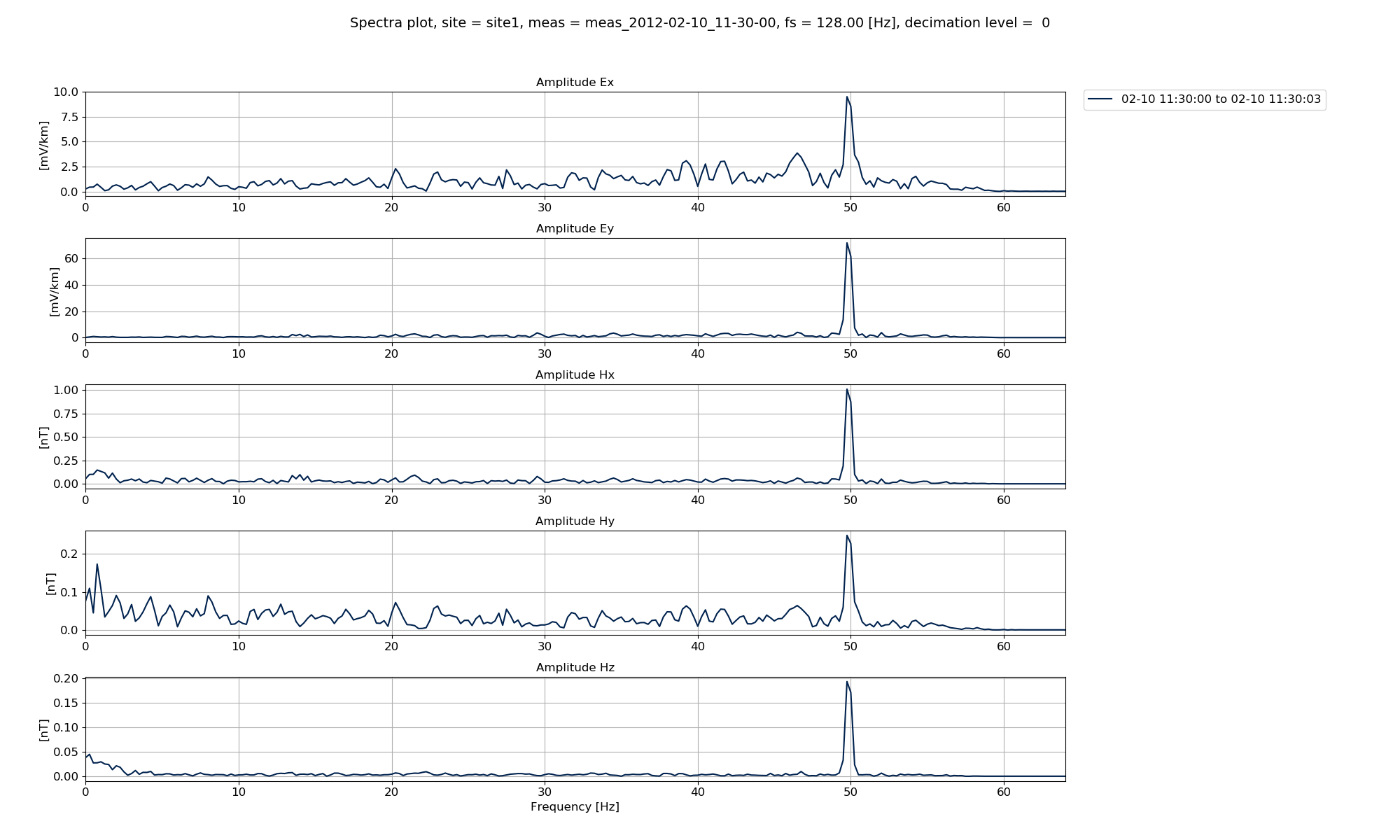
Default spectra data
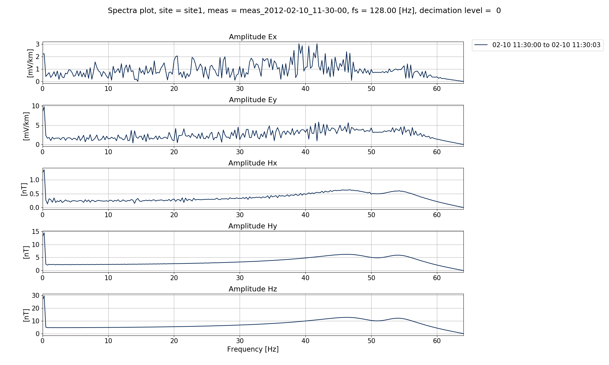
Notched spectra data
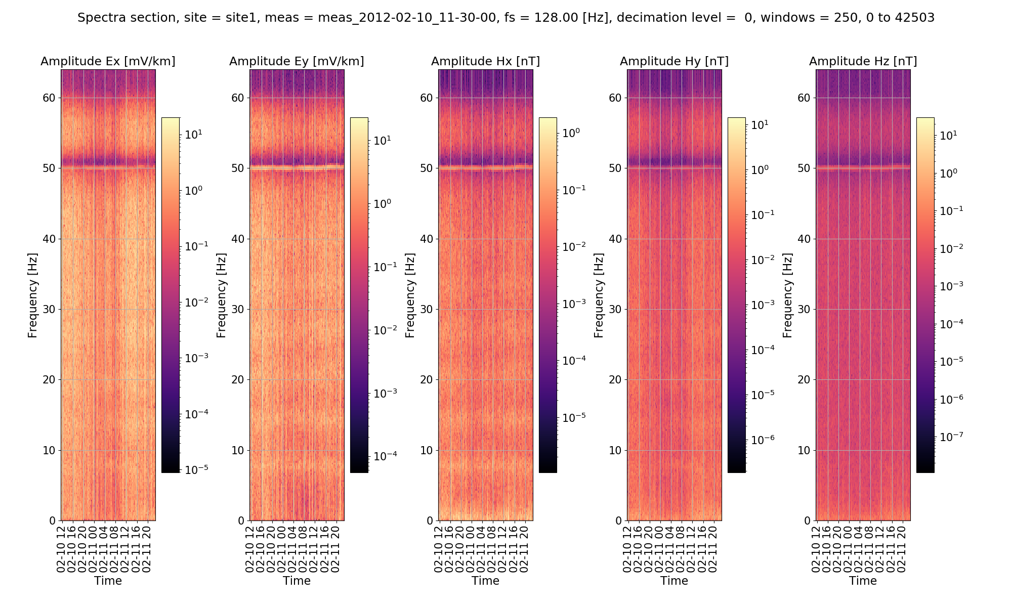
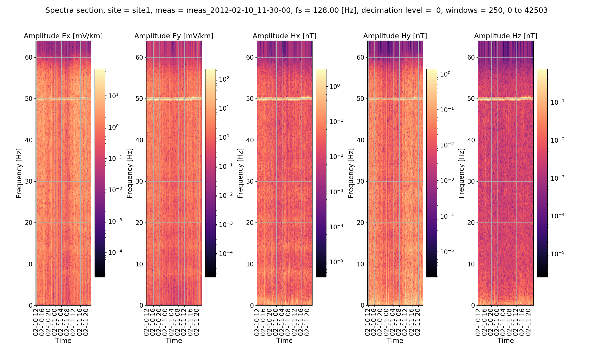
A spectra section can also be plotted in a similar to way the example shown in Viewing Spectra.
28 29 30 31 32 33 34 35 36 37 | fig = viewSpectraSection(
projData,
"site1",
"meas_2012-02-10_11-30-00",
specdir="notch",
plotoptions=plotOptions,
show=False,
save=False,
)
fig.savefig(imagePath / "multspec_viewspec_notch_section")
|
Notched spectra section
For the sake of comarpison, the default (no notch) spectra section.
Default spectra section
Further, inspecting the comments of the notched spectra data, the application of the notch filter and the frequency is recorded.
1 2 3 4 5 6 7 8 9 10 11 12 13 14 15 16 17 18 19 20 21 22 23 24 25 26 27 28 29 30 31 32 33 34 35 36 37 | Unscaled data 2012-02-10 11:30:00 to 2012-02-11 23:03:43.992188 read in from measurement E:\magnetotellurics\code\resisticsdata\tutorial\tutorialProject\timeData\site1\meas_2012-02-10_11-30-00, samples 0 to 16387071
Sampling frequency 128.0
Scaling channel Ex with scalar -0.000112591 to give mV
Dividing channel Ex by electrode distance 0.08 km to give mV/km
Scaling channel Ey with scalar -0.000112512 to give mV
Dividing channel Ey by electrode distance 0.091 km to give mV/km
Scaling channel Hx with scalar -0.00360174 to give mV
Scaling channel Hy with scalar -0.00360038 to give mV
Scaling channel Hz with scalar -0.0036007 to give mV
Remove zeros: False, remove nans: False, remove average: True
---------------------------------------------------
Calculating project spectra
Using default configuration
Channel Ex not calibrated
Channel Ey not calibrated
Channel Hx calibrated with calibration data from file E:\magnetotellurics\code\resisticsdata\tutorial\tutorialProject\calData\Hx_MFS06365.TXT
Channel Hy calibrated with calibration data from file E:\magnetotellurics\code\resisticsdata\tutorial\tutorialProject\calData\Hy_MFS06357.TXT
Channel Hz calibrated with calibration data from file E:\magnetotellurics\code\resisticsdata\tutorial\tutorialProject\calData\Hz_MFS06307.TXT
Notch filter applied at 50 Hz
Decimating with 7 levels and 7 frequencies per level
Evaluation frequencies for this level 32.0, 22.62741699796952, 16.0, 11.31370849898476, 8.0, 5.65685424949238, 4.0
Windowing with window size 512 samples and overlap 128 samples
Time data decimated from 128.0 Hz to 16.0 Hz, new start time 2012-02-10 11:30:00, new end time 2012-02-11 23:03:43.937500
Evaluation frequencies for this level 2.82842712474619, 2.0, 1.414213562373095, 1.0, 0.7071067811865475, 0.5, 0.35355339059327373
Windowing with window size 512 samples and overlap 128 samples
Time data decimated from 16.0 Hz to 2.0 Hz, new start time 2012-02-10 11:30:00, new end time 2012-02-11 23:03:43.500000
Evaluation frequencies for this level 0.25, 0.17677669529663687, 0.125, 0.08838834764831843, 0.0625, 0.044194173824159216, 0.03125
Windowing with window size 512 samples and overlap 128 samples
Time data decimated from 2.0 Hz to 0.25 Hz, new start time 2012-02-10 11:30:00, new end time 2012-02-11 23:03:40
Time data decimated from 0.25 Hz to 0.125 Hz, new start time 2012-02-10 11:30:00, new end time 2012-02-11 23:03:36
Evaluation frequencies for this level 0.022097086912079608, 0.015625, 0.011048543456039804, 0.0078125, 0.005524271728019902, 0.00390625, 0.002762135864009951
Windowing with window size 512 samples and overlap 128 samples
Time data decimated from 0.125 Hz to 0.015625 Hz, new start time 2012-02-10 11:30:00, new end time 2012-02-11 23:03:20
Evaluation frequencies for this level 0.001953125, 0.0013810679320049755, 0.0009765625, 0.0006905339660024878, 0.00048828125, 0.0003452669830012439, 0.000244140625
Windowing with window size 512 samples and overlap 128 samples
Spectra data written out to E:\magnetotellurics\code\resisticsdata\tutorial\tutorialProject\specData\site1\meas_2012-02-10_11-30-00\notch on 2019-10-05 20:10:06.845930 using resistics 0.0.6.dev2
---------------------------------------------------
|
The next step is to process the notched spectra data. To do this, specdir has to be specified in the call to processProject() as shown below:
39 40 41 42 | # process the new set of spectra
from resistics.project.transfunc import processProject
processProject(projData, sites=["site1"], specdir="notch")
|
Finally, the transfer function data for the notched spectra data can be viewed by once more specifying the specdir option in the call to viewImpedance()
44 45 46 47 48 49 50 51 52 53 54 55 56 57 58 59 60 61 62 63 64 65 66 67 68 | # plot the transfer functions, again with specifying the relevant specdir
from resistics.project.transfunc import viewImpedance
figs = viewImpedance(
projData,
sites=["site1"],
sampleFreqs=[128],
oneplot=False,
specdir="notch",
save=False,
show=False,
)
figs[0].savefig(imagePath / "multspec_viewimp_notch")
# and compare to the original
figs = viewImpedance(
projData,
sites=["site1"],
sampleFreqs=[128],
oneplot=False,
specdir="spectra",
save=False,
show=False,
)
figs[0].savefig(imagePath / "multspec_viewimp_nonotch")
|
The impedance for the default spectra calculated parameters and then for the notch parameters are shown below.
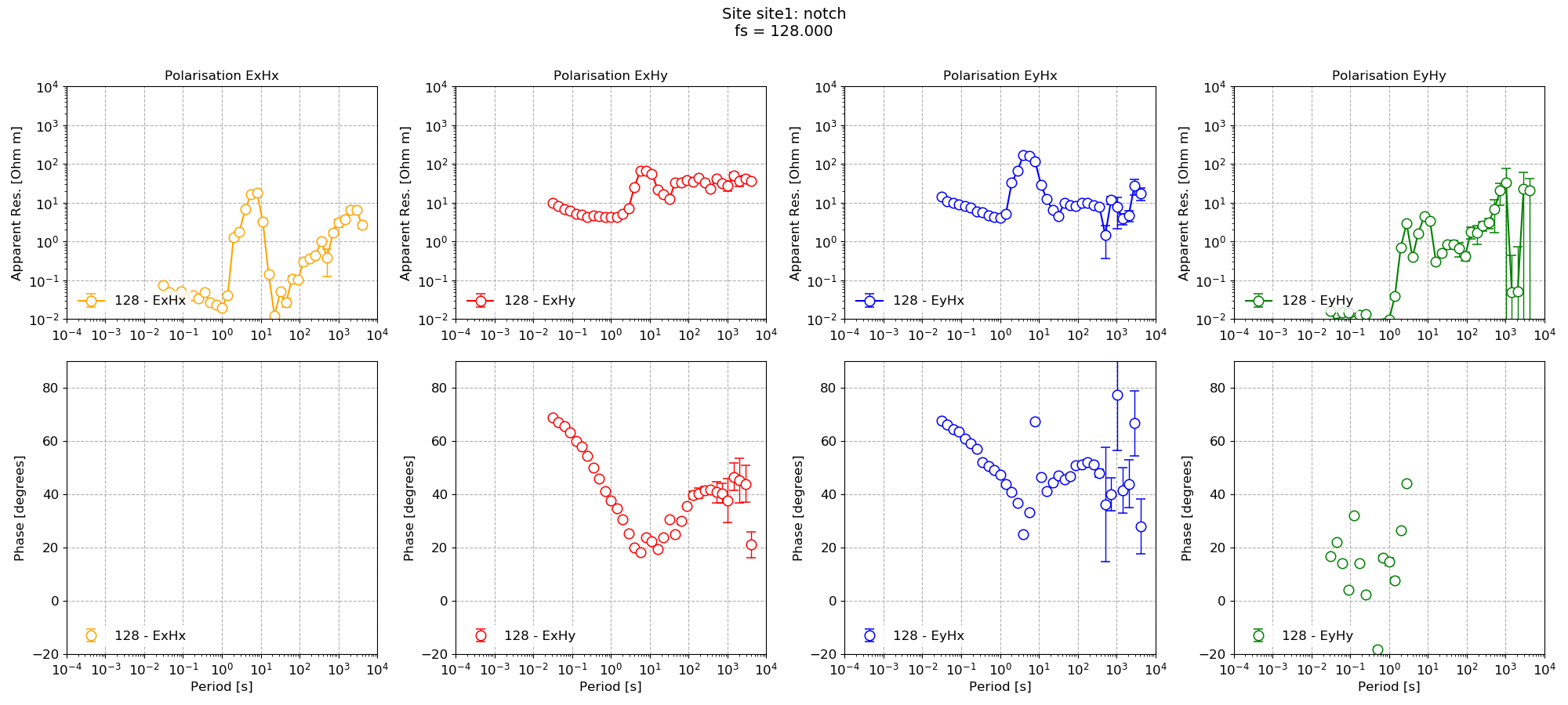
Default impedance tensor estimation
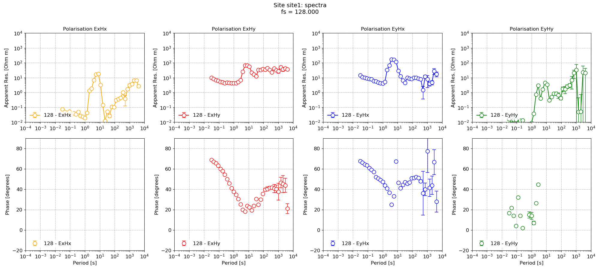
Impedance tensor estimation using the notched spectra data
As mentioned in the note at the top of this page, the simplest way to use the specdir option is through configuration files.
Important
When specifying specdir in a configuration file, the specdir keyword no longer has to be passed to the various method calls as it is picked up directly from the confiugration file. This makes everything much simpler and removes a source of mistakes.
More information about configuration files is provided in the Configuration files section. An example of using configuration files is provided in the Using configuration files section.
Complete example script
For the purposes of clarity, the complete example script is provided below.
1 2 3 4 5 6 7 8 9 10 11 12 13 14 15 16 17 18 19 20 21 22 23 24 25 26 27 28 29 30 31 32 33 34 35 36 37 38 39 40 41 42 43 44 45 46 47 48 49 50 51 52 53 54 55 56 57 58 59 60 61 62 63 64 65 66 67 68 | from datapaths import projectPath, imagePath
from resistics.project.io import loadProject
projData = loadProject(projectPath)
# calculate another set of spectra for the 128 Hz data with notching at 50Hz and 16.667Hz
from resistics.project.spectra import calculateSpectra
calculateSpectra(projData, sampleFreqs=[128], notch=[50], specdir="notch")
projData.refresh()
# view the spectra
from resistics.common.plot import plotOptionsSpec, getPaperFonts
from resistics.project.spectra import viewSpectra, viewSpectraSection

plotOptions = plotOptionsSpec(plotfonts=getPaperFonts())
fig = viewSpectra(
    projData,
    "site1",
    "meas_2012-02-10_11-30-00",
    specdir="notch",
    plotoptions=plotOptions,
    show=False,
    save=False,
)
fig.savefig(imagePath / "multspec_viewspec_notch_spec")
fig = viewSpectraSection(
    projData,
    "site1",
    "meas_2012-02-10_11-30-00",
    specdir="notch",
    plotoptions=plotOptions,
    show=False,
    save=False,
)
fig.savefig(imagePath / "multspec_viewspec_notch_section")
# process the new set of spectra
from resistics.project.transfunc import processProject

processProject(projData, sites=["site1"], specdir="notch")
# plot the transfer functions, again with specifying the relevant specdir
from resistics.project.transfunc import viewImpedance

figs = viewImpedance(
    projData,
    sites=["site1"],
    sampleFreqs=[128],
    oneplot=False,
    specdir="notch",
    save=False,
    show=False,
)
figs[0].savefig(imagePath / "multspec_viewimp_notch")

# and compare to the original
figs = viewImpedance(
    projData,
    sites=["site1"],
    sampleFreqs=[128],
    oneplot=False,
    specdir="spectra",
    save=False,
    show=False,
)
figs[0].savefig(imagePath / "multspec_viewimp_nonotch")
|