Up and running
Resistics can quickly run projects with default settings by using the project API. Default configuration options are detailed in Configuration parameters section.
Begin by loading the project and calculating spectra. Spectra can be batch calculated using the calculateSpectra() method in spectra. The are several options for calculating spectra, which are detailed in the API documentation.
1 2 3 4 5 6 7 8 9 10 11 | from datapaths import projectPath, imagePath
from resistics.project.io import loadProject
# load the project
projData = loadProject(projectPath)
# calculate spectrum using standard options
from resistics.project.spectra import calculateSpectra
calculateSpectra(projData)
projData.refresh()
|
Note
After calculating spectra, it is best practice to refresh the project to make sure everything is picked up.
Spectra data files are stored in project specData directory. The folder structure is similar to the timeData folder
exampleProject
├── calData
├── timeData
│   └── site1
|       |── dataFolder1
│       |── dataFolder2
|       |──     .
|       |──     .
|       |──     .
|       └── dataFolderN
├── specData
│   └── site1
|       |── dataFolder1
|       |   └── spectra
│       |── dataFolder2
|       |   └── spectra
|       |──     .
|       |──     .
|       |──     .
|       └── dataFolderN
|           └── spectra
├── statData
├── maskData
├── transFuncData
├── images
└── mtProj.prj
By default spectra are stored in a folder called spectra under the dataFolder. The reason for this will become clearer in the section covering multiple spectra.
The next step is to process the spectra to estimate the impedance tensor. This is done using the processProject() method in project transfunc module.
13 14 15 16 | # process the spectra
from resistics.project.transfunc import processProject
processProject(projData)
|
Transfer function data is stored under the transFuncData folder as shown below. As transfer functions are calculated out for each unique sampling frequency in a site, the data is stored with respect to sampling frequencies.
exampleProject
├── calData
├── timeData
│ └── site1
| |── dataFolder1
│ |── dataFolder2
| |── .
| |── .
| |── .
| └── dataFolderN
├── specData
│ └── site1
| |── dataFolder1
| | └── spectra
│ |── dataFolder2
| | └── spectra
| |── .
| |── .
| |── .
| └── dataFolderN
| └── spectra
├── statData
├── maskData
├── transFuncData
│ └── site1
| |── sampling frequency (e.g. 128)
│ └── sampling frequency (e.g. 4096)
├── images
└── mtProj.prj
Transfer functions are saved in an internal format. This is a minimal format currently and could possibly be amended in the future. An example transfer function data file is given below.
1 2 3 4 5 6 7 8 9 10 11 12 13 14 15 16 17 18 19 20 21 22 23 24 25 | sampleFreq = 128.0
insite = site1
inchans = Hx, Hy
outsite = site1
outchans = Ex, Ey
remotesite = False
remotechans = False
Evaluation frequencies
32.00000000, 22.62741700, 16.00000000, 11.31370850, 8.00000000, 5.65685425, 4.00000000, 2.82842712, 2.00000000, 1.41421356, 1.00000000, 0.70710678, 0.50000000, 0.35355339, 0.25000000, 0.17677670, 0.12500000, 0.08838835, 0.06250000, 0.04419417, 0.03125000, 0.02209709, 0.01562500, 0.01104854, 0.00781250, 0.00552427, 0.00390625, 0.00276214, 0.00195312, 0.00138107, 0.00097656, 0.00069053, 0.00048828, 0.00034527, 0.00024414
Z-ExHx
0.94934095+3.34752925j, 0.39757620+2.31074358j, 0.52617285+1.72688405j, 0.57151994+1.62066209j, 0.42465600+1.08405030j, 0.46637822+0.96810741j, 0.32503341+0.76018855j, 0.24331743+0.80425821j, 0.06035649+0.52144572j, -0.02926691+0.40388910j, -0.00388458+0.31499819j, 0.14867030+0.35651599j, 1.25343444+1.30843791j, 1.24952015+1.30422883j, 2.00530716+2.14396892j, 2.54738388+2.87838374j, 2.44286873+2.32328446j, 0.91499849+0.77452574j, 0.15529015+0.14187726j, 0.04168938-0.03179742j, 0.08489140-0.02836873j, 0.04885159-0.02570243j, 0.08177452-0.04471374j, 0.06060611-0.04559944j, 0.10969232-0.00633376j, 0.09870060-0.01672921j, 0.09291384-0.00253664j, 0.11843436-0.01170368j, 0.06017847-0.01214193j, 0.10720693-0.00774427j, 0.12193016-0.00049235j, 0.10775218-0.03415012j, 0.12406724+0.01289080j, 0.10033646+0.03319441j, 0.05015572+0.02673676j
Z-ExHy
-14.49940719-37.30760221j, -11.70449296-27.92094103j, -9.58646483-21.24857056j, -8.49393124-16.84212160j, -7.20648741-12.55985294j, -6.25007072-10.00469866j, -5.35440757-7.48059143j, -5.27749416-6.28817269j, -4.64835243-4.80556616j, -4.13984011-3.62145882j, -3.64050425-2.82249255j, -3.20538184-2.21126072j, -3.06869371-1.82345205j, -3.15032118-1.48575721j, -5.27539185-1.91007092j, -7.28040263-2.40627879j, -5.91484112-2.62165093j, -4.58620313-1.89011797j, -2.47789077-0.88026086j, -1.75718710-0.77247855j, -1.20738839-0.71370142j, -1.74518887-0.81418400j, -1.37795934-0.79292303j, -1.17302197-0.83596754j, -0.88585041-0.73593556j, -0.83052943-0.70764570j, -0.60677629-0.53702043j, -0.41997441-0.37361064j, -0.47871823-0.41321326j, -0.35261010-0.30032226j, -0.29039855-0.22477508j, -0.28698712-0.30366764j, -0.21189162-0.21371479j, -0.19227688-0.18486923j, -0.19590496-0.07540370j
Z-EyHx
18.20900983+44.19330179j, 14.25977483+32.32255518j, 12.00673840+25.16266292j, 10.18581044+20.42077827j, 8.74051642+15.68524229j, 7.51782581+12.65223294j, 5.96526157+9.17549622j, 5.48179656+7.03026378j, 4.30551261+5.26439927j, 3.56099277+4.13318961j, 3.06957170+3.32893354j, 3.06223840+2.94061316j, 6.84027528+5.91975520j, 8.73552808+6.53555433j, 13.24324129+6.21611655j, 9.91018097+6.47104007j, 3.28067547+7.90417386j, 2.48747630+2.61294003j, 1.47097830+1.29084507j, 0.84798061+0.82853610j, 0.57728301+0.61977038j, 0.72974858+0.74302537j, 0.56744520+0.60411131j, 0.42885723+0.52804983j, 0.38582516+0.47965379j, 0.31921721+0.40909345j, 0.25536429+0.31891899j, 0.22080524+0.24509160j, 0.09676873+0.07074661j, 0.21789833+0.18302424j, 0.04294983+0.19052502j, 0.08708353+0.07699017j, 0.07675592+0.07402667j, 0.08673723+0.20196350j, 0.12931911+0.06841353j
Z-EyHy
1.53272103+0.46507243j, 0.88238966+0.35168425j, 1.04668728+0.26176702j, 0.91239160+0.06634902j, 0.50165189+0.31376583j, 0.58690792+0.14762767j, 0.52133177+0.01975289j, 0.08411439-0.30004512j, 0.18691456-0.08718443j, 0.21232617+0.05635269j, 0.20271085+0.05071919j, 0.36167486+0.04487767j, 1.19861804+0.59566704j, 1.61679145+1.60715819j, -0.19352520+0.67781159j, -1.18731922+0.20772039j, 0.42284310-1.61757173j, -1.01697784-0.68199125j, 0.27228105+0.15062302j, 0.29178195+0.16189748j, 0.30222784+0.20253571j, 0.22943737+0.19933146j, 0.17789543+0.14104224j, 0.08393666+0.12636427j, 0.15642692+0.21188491j, 0.01618003+0.21544456j, 0.06226938+0.21412314j, 0.07889024+0.19004886j, 0.13997257-0.21366792j, 0.25915111+0.27144077j, -0.32782421+0.23635934j, 0.01056732-0.00763337j, 0.00838169+0.00764168j, -0.02318327+0.19745418j, 0.15469331-0.03335532j
Var-ExHx
0.00000273, 0.00000317, 0.00000290, 0.00000156, 0.00000079, 0.00000005, 0.00000000, 0.00000005, 0.00000003, 0.00000002, 0.00000001, 0.00000001, 0.00000000, 0.00000000, 0.00000058, 0.00000035, 0.00000013, 0.00000003, 0.00000002, 0.00000002, 0.00000005, 0.00002685, 0.00003132, 0.00001009, 0.00001954, 0.00002070, 0.00001109, 0.00000553, 0.00021954, 0.00003812, 0.00011019, 0.00007752, 0.00005389, 0.00004420, 0.00001575
Var-ExHy
0.00000282, 0.00000323, 0.00000327, 0.00000127, 0.00000131, 0.00000040, 0.00000025, 0.00005430, 0.00005796, 0.00005538, 0.00005276, 0.00004405, 0.00000910, 0.00000089, 0.00009786, 0.00007130, 0.00002502, 0.00000632, 0.00000288, 0.00000069, 0.00000041, 0.00029772, 0.00045784, 0.00008764, 0.00043093, 0.00064663, 0.00023288, 0.00006586, 0.00097159, 0.00045125, 0.00147858, 0.00072224, 0.00100352, 0.00054187, 0.00016173
Var-EyHx
0.00000453, 0.00000662, 0.00000558, 0.00000245, 0.00000102, 0.00000005, 0.00000000, 0.00000006, 0.00000004, 0.00000003, 0.00000002, 0.00000001, 0.00000001, 0.00000000, 0.00000245, 0.00000074, 0.00000025, 0.00000004, 0.00000003, 0.00000003, 0.00000007, 0.00006678, 0.00006971, 0.00002173, 0.00004459, 0.00005035, 0.00002393, 0.00003852, 0.00105869, 0.00051077, 0.00260490, 0.00015475, 0.00014732, 0.00113611, 0.00036592
Var-EyHy
0.00000468, 0.00000675, 0.00000630, 0.00000199, 0.00000169, 0.00000045, 0.00000033, 0.00006856, 0.00007873, 0.00007864, 0.00007831, 0.00006894, 0.00003272, 0.00000537, 0.00041467, 0.00015222, 0.00004976, 0.00000741, 0.00000393, 0.00000114, 0.00000063, 0.00074045, 0.00101918, 0.00018877, 0.00098339, 0.00157321, 0.00050255, 0.00045890, 0.00468527, 0.00604659, 0.03495500, 0.00144177, 0.00274341, 0.01392825, 0.00375633
|
The reason to use this rather than EDI for now is an intention to build this out further to include more information about uncertainty that can be taken further into an inversion process.
Once the components of the impedance tensor have been calculated, it is possible to visualise them using the viewImpedance() method available in the transfunc module.
18 19 20 21 22 | # plot transfer function and save the plot
from resistics.project.transfunc import viewImpedance
figs = viewImpedance(projData, sites=["site1"], show=False, save=False)
figs[0].savefig(imagePath / "simpleRun_viewimp_default")
|
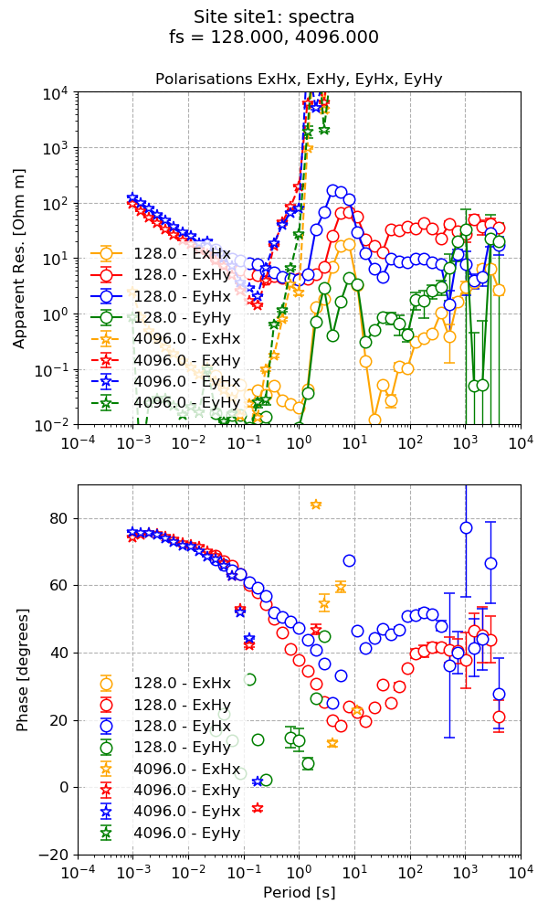
The default plot for transfer functions
However, this plot is quite busy. One way to simplify the plot is to explicitly specify the polarisations to plot.
24 25 26 27 28 | # or keep the two most important polarisations on the same plot
figs = viewImpedance(
projData, sites=["site1"], polarisations=["ExHy", "EyHx"], save=False, show=False
)
figs[0].savefig(imagePath / "simpleRun_viewimp_polarisations")
|
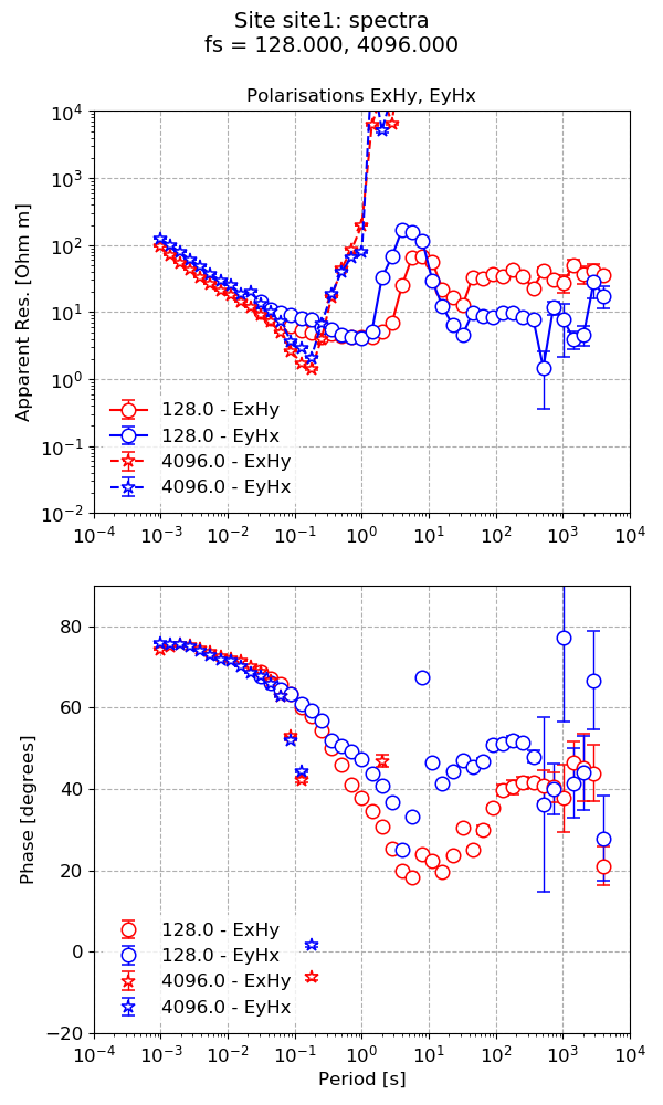
Limiting the polarisations in a transfer function plot
On occasion, it can be more useful to plot each component separately. This can be done by setting oneplot = False in the arguments.
30 31 32 | # this plot is quite busy, let's plot all the components on separate plots
figs = viewImpedance(projData, sites=["site1"], oneplot=False, save=False, show=False)
figs[0].savefig(imagePath / "simpleRun_viewimp_multplot")
|
This results in the following plot.
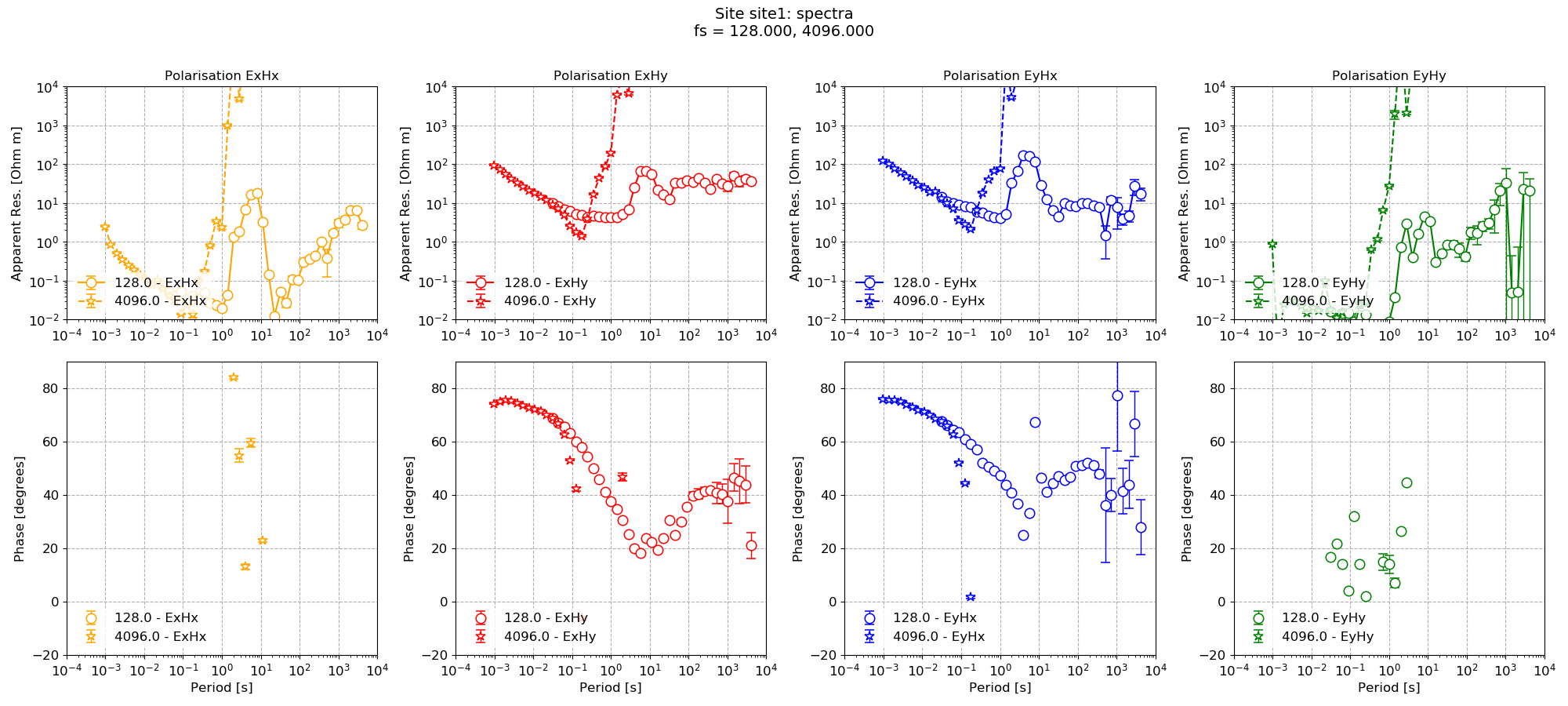
Polarisations of impedance tensor plotted on separate plots
To read in a transfer function directly, the getTransferFunctionData() method of the transfunc module can be used. The getTransferFunctionData() will read in the transfer function data file and return a TransferFunctionData object with information about the components of the transfer function data.
34 35 36 37 | # get a transfer function data object
from resistics.project.transfunc import getTransferFunctionData
tfData = getTransferFunctionData(projData, "site1", 128)
|
Warning
Currently, resistics uses a proprietry, but still ASCII, transfer function file format. As .edi files are the standard format for magnetotellurics, these will be properly supported going forwards. However, the intention with current file format is to allow for additional future changes that capture more information that would be useful for geophysical inversion.
The transfer function data can be plotted using the view() method of TransferFunctionData. This is shown below, along with the plot.
38 39 | fig = tfData.viewImpedance(oneplot=True, polarisations=["ExHy", "EyHx"], save=True)
fig.savefig(imagePath / "simpleRun_tfData_view")
|
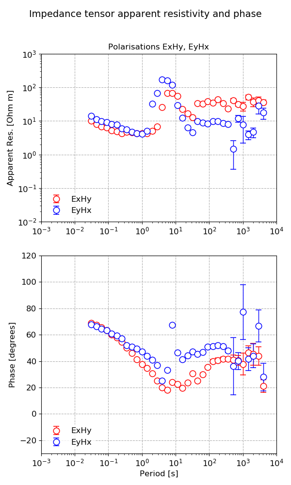
Plotting the transfer function data individually
Complete example script
For clarity, the complete example script is provided below.
1 2 3 4 5 6 7 8 9 10 11 12 13 14 15 16 17 18 19 20 21 22 23 24 25 26 27 28 29 30 31 32 33 34 35 36 37 38 39 | from datapaths import projectPath, imagePath
from resistics.project.io import loadProject
# load the project
projData = loadProject(projectPath)
# calculate spectrum using standard options
from resistics.project.spectra import calculateSpectra
calculateSpectra(projData)
projData.refresh()
# process the spectra
from resistics.project.transfunc import processProject

processProject(projData)
# plot transfer function and save the plot
from resistics.project.transfunc import viewImpedance

figs = viewImpedance(projData, sites=["site1"], show=False, save=False)
figs[0].savefig(imagePath / "simpleRun_viewimp_default")
# or keep the two most important polarisations on the same plot
figs = viewImpedance(
    projData, sites=["site1"], polarisations=["ExHy", "EyHx"], save=False, show=False
)
figs[0].savefig(imagePath / "simpleRun_viewimp_polarisations")
# this plot is quite busy, let's plot all the components on separate plots
figs = viewImpedance(projData, sites=["site1"], oneplot=False, save=False, show=False)
figs[0].savefig(imagePath / "simpleRun_viewimp_multplot")
# get a transfer function data object
from resistics.project.transfunc import getTransferFunctionData

tfData = getTransferFunctionData(projData, "site1", 128)
fig = tfData.viewImpedance(oneplot=True, polarisations=["ExHy", "EyHx"], save=True)
fig.savefig(imagePath / "simpleRun_tfData_view")
|