Calculating the tipper
The tipper is the transfer function between the input horizontal magnetic fields, Hx and Hy, and the output vertical magnetic field, Hz. It is complex-valued like the impedance tensor and describes the tipping of the magnetic field out of the horizontal plane.
By default, resistics does not calculate the components of the tipper. This is because resistics sets the default input channels as Hx and Hy and the default output channels as Ex and Ey.
There are two options for calculating the tipper:
The first is to add Hz as one of the output channels in the transfer function calculation
The second is to set Hz as the only output channel
The first option sets up the following linear equations to be solved in the linear regression:
The second can be understood as solving only:
These will pribably both give slightly different solutions for the tipper components as the optimal solution for the robust regression will vary between them.
Warning
Including Hz as one of the output channels with Ex and Ey will likely give slightly different results for Zxy, Zxx, Zyx and Zyy than when the it is excluded. This is due to changing the nature of the robust regression.
Continuing on from the example in the previous section, the spectra have already been calculated and it is possible to simply process the same spectra again, but this time using different input and output channels. However, to avoid overwriting the previously calculated transfer function, pass postpend=”with_Hz” to processProject(). The postpend is simply a string that is concantenated to the end of the transfer function data file.
1 2 3 4 5 6 7 8 9 10 11 12 | from datapaths import projectPath, imagePath
from resistics.project.io import loadProject
# load the project
projData = loadProject(projectPath)
# process the spectra with tippers
from resistics.project.transfunc import processProject
processProject(
projData, sites=["site1"], outchans=["Ex", "Ey", "Hz"], postpend="with_Hz"
)
|
The output transfer function data file looks like this.
1 2 3 4 5 6 7 8 9 10 11 12 13 14 15 16 17 18 19 20 21 22 23 24 25 26 27 28 29 30 31 32 33 | sampleFreq = 128.0
insite = site1
inchans = Hx, Hy
outsite = site1
outchans = Ex, Ey, Hz
remotesite = False
remotechans = False
Evaluation frequencies
32.00000000, 22.62741700, 16.00000000, 11.31370850, 8.00000000, 5.65685425, 4.00000000, 2.82842712, 2.00000000, 1.41421356, 1.00000000, 0.70710678, 0.50000000, 0.35355339, 0.25000000, 0.17677670, 0.12500000, 0.08838835, 0.06250000, 0.04419417, 0.03125000, 0.02209709, 0.01562500, 0.01104854, 0.00781250, 0.00552427, 0.00390625, 0.00276214, 0.00195312, 0.00138107, 0.00097656, 0.00069053, 0.00048828, 0.00034527, 0.00024414
Z-ExHx
1.04079186+3.29654452j, 0.53027757+2.29615963j, 0.60747306+1.72368328j, 0.64591267+1.58412509j, 0.45353802+1.09436451j, 0.51521582+0.95449169j, 0.36101811+0.76557261j, 0.28401122+0.84424910j, 0.10112565+0.53929264j, -0.00386989+0.43660320j, -0.00188984+0.32691375j, 1.12548929+1.37565672j, 1.15410649+1.10868840j, 1.16370598+0.98670410j, 1.87562019+2.43647685j, 3.05608851+2.16112275j, 2.19440338+2.10424919j, 0.73063466+0.73102177j, 0.14258188+0.13986741j, 0.04077148-0.03765126j, 0.09175197-0.02720623j, 0.05974526-0.05196585j, 0.07693643-0.04907649j, 0.05961643-0.05890145j, 0.11272858-0.01144124j, 0.09865408-0.03202689j, 0.10253566-0.03349029j, 0.12542555-0.03286090j, 0.07033758+0.02210766j, 0.10930044+0.00464463j, 0.10268325+0.02065984j, 0.09936503-0.00253428j, 0.11968035-0.00215333j, 0.10947036+0.02374593j, 0.04939511+0.03412870j
Z-ExHy
-14.77622870-37.31129331j, -11.94204138-27.92099933j, -9.82263792-21.21887914j, -8.63782128-16.77992300j, -7.31524564-12.54817916j, -6.31606883-9.99251927j, -5.39071181-7.48158779j, -5.33541577-6.28759974j, -4.70052449-4.81326698j, -4.21590597-3.64801070j, -3.72529494-2.86313281j, -3.13304663-2.12457585j, -2.70387756-1.58268163j, -2.46811141-1.15204490j, -5.81048438-2.03744524j, -4.38793537-1.69521640j, -3.74770903-1.91769754j, -5.09815714-1.84136397j, -2.94490309-0.99680297j, -1.76236388-0.74490585j, -1.14469788-0.68123925j, -1.53502456-0.77134555j, -1.38173130-0.80358146j, -1.19098376-0.91004351j, -0.81896453-0.70268955j, -0.76471674-0.69119026j, -0.52108343-0.55435015j, -0.36433996-0.38777994j, -0.51103758-0.34560385j, -0.36920419-0.27194357j, -0.36949651-0.18846234j, -0.31160864-0.21790788j, -0.27906831-0.26769807j, -0.20049858-0.25688384j, -0.18964245-0.07565621j
Z-EyHx
18.37007150+44.34198117j, 14.48579815+32.63219293j, 12.14913379+25.27990840j, 10.24730560+20.41950063j, 8.78360394+15.70300190j, 7.56534895+12.69301556j, 6.01903388+9.26191548j, 5.58395322+7.28768554j, 4.39691114+5.40627620j, 3.58585839+4.16744819j, 3.06034922+3.31287318j, 6.25958904+6.12078856j, 6.30087543+5.47987197j, 8.18096119+5.76850532j, 4.57778513+2.32932350j, 4.12760665+2.41015659j, 1.80862482+1.85166020j, 2.06175341+2.25296853j, 1.54955421+1.34323284j, 0.84100660+0.81317173j, 0.56677533+0.61182987j, 0.72058152+0.72347561j, 0.55899271+0.60001061j, 0.42946626+0.52859905j, 0.38449672+0.46939549j, 0.31868606+0.38099839j, 0.22472007+0.23009283j, 0.21086045+0.20210333j, 0.21235825+0.19804087j, 0.23798696+0.15141392j, -0.04338280+0.15087016j, 0.07165787+0.07542711j, 0.08030578+0.09552357j, 0.14267848+0.18085567j, 0.08371758+0.04627095j
Z-EyHy
1.35920615+0.53877795j, 0.78943313+0.43424079j, 0.89834838+0.32491324j, 0.78545940+0.11770502j, 0.42246412+0.33654264j, 0.52416697+0.17188427j, 0.48705399+0.03440855j, 0.07174323-0.32128346j, 0.19182482-0.11077581j, 0.22423973+0.03783523j, 0.20693075+0.04996355j, 0.73731876+0.30827521j, 0.98749960+0.55182081j, 1.95532366+2.07140558j, -1.24176242-0.56542653j, -1.51464861-0.64543660j, -0.65149673-0.95543067j, -0.64036311-0.54455918j, 0.30127514+0.23398902j, 0.30272748+0.22348305j, 0.37532464+0.29250416j, 0.28539855+0.19760767j, 0.18955759+0.18742306j, 0.12054101+0.15317445j, 0.23363038+0.25125289j, 0.16414092+0.25139784j, 0.14801336+0.04343296j, 0.16452941+0.10480170j, 0.17246646+0.11916276j, 0.37351748+0.25451382j, -0.51266710+0.01373046j, -0.02616416+0.01216457j, 0.05861090+0.11035731j, 0.12006981+0.01000948j, 0.13528802-0.01430632j
Z-HzHx
0.01755160+0.00381437j, 0.01714836+0.00295434j, 0.01833738+0.00320913j, 0.01775372+0.00501416j, 0.01733679+0.00956355j, 0.01073518+0.00931466j, 0.00404209+0.00392591j, 0.00438347-0.02285013j, 0.01639262-0.01025608j, 0.02186220-0.00164491j, 0.02471828+0.00847618j, 0.02009220+0.01776959j, 0.00946444+0.01407880j, -0.00712147+0.01987152j, -0.01119215+0.01513196j, -0.01800915+0.00357674j, -0.02489738+0.00953308j, -0.02058911+0.00445469j, -0.03767142-0.02032189j, -0.02294150+0.00181478j, -0.02279655+0.00836583j, -0.00804860+0.00309415j, -0.00549625+0.01558853j, -0.05288059+0.04088519j, -0.07927733+0.02220952j, -0.04961333-0.00720804j, -0.05291897-0.02660196j, -0.02742707-0.04626052j, 0.37834186-0.27432165j, 0.04101920-0.12329491j, 0.07078130-0.14471890j, 0.18143447-0.02777018j, 0.15875579+0.01484287j, -0.05482596+0.11928385j, -0.21790014-0.09902028j
Z-HzHy
-0.00647873-0.02118345j, -0.00477559-0.02706761j, -0.00281663-0.03734579j, 0.00416165-0.05106725j, 0.02019722-0.06706969j, 0.03984897-0.08045074j, 0.07087277-0.08826900j, 0.15246688-0.14039695j, 0.16953066-0.10506934j, 0.19290846-0.08031194j, 0.22009794-0.05594914j, 0.23589998-0.02738644j, 0.24562599-0.00005751j, 0.16395687+0.02060615j, 0.16768765+0.04141987j, 0.16322932+0.05133452j, 0.13222024+0.05000424j, 0.09608473+0.03131385j, 0.20084086+0.05172580j, 0.17987058-0.01355505j, 0.16878988-0.03922035j, 0.18402722-0.03298401j, 0.20046778-0.04022156j, 0.08166815+0.01401893j, 0.05672439-0.02595539j, 0.15976216-0.04557310j, 0.13302815-0.06553806j, 0.17154298-0.09200181j, 0.94848115+0.02413481j, 0.31146772-0.19029895j, 0.50251785-0.30776092j, 0.67150704-0.01101146j, 0.77688396-0.08610456j, 0.63856137+0.32008258j, -1.35822274+0.25495992j
Var-ExHx
0.00000035, 0.00000047, 0.00000048, 0.00000032, 0.00000017, 0.00000001, 0.00000000, 0.00000001, 0.00000001, 0.00000001, 0.00000000, 0.00000000, 0.00000000, 0.00000000, 0.00000033, 0.00000010, 0.00000004, 0.00000002, 0.00000001, 0.00000001, 0.00000002, 0.00001724, 0.00001626, 0.00000498, 0.00001018, 0.00000798, 0.00000467, 0.00000241, 0.00041598, 0.00012366, 0.00018874, 0.00009119, 0.00012613, 0.00010849, 0.00001487
Var-ExHy
0.00000036, 0.00000048, 0.00000054, 0.00000026, 0.00000028, 0.00000010, 0.00000007, 0.00001385, 0.00001538, 0.00001524, 0.00001584, 0.00002227, 0.00000342, 0.00000033, 0.00003877, 0.00001428, 0.00000584, 0.00000262, 0.00000137, 0.00000030, 0.00000014, 0.00019110, 0.00023771, 0.00004323, 0.00022424, 0.00024844, 0.00009789, 0.00002856, 0.00181491, 0.00144813, 0.00252695, 0.00084748, 0.00234161, 0.00125569, 0.00011658
Var-EyHx
0.00000061, 0.00000097, 0.00000092, 0.00000051, 0.00000023, 0.00000001, 0.00000000, 0.00000001, 0.00000001, 0.00000001, 0.00000001, 0.00000001, 0.00000000, 0.00000000, 0.00000028, 0.00000009, 0.00000002, 0.00000002, 0.00000001, 0.00000002, 0.00000004, 0.00002234, 0.00002202, 0.00000862, 0.00001719, 0.00001952, 0.00000766, 0.00001202, 0.00036835, 0.00039727, 0.00123595, 0.00015289, 0.00009368, 0.00039567, 0.00046637
Var-EyHy
0.00000063, 0.00000099, 0.00000104, 0.00000042, 0.00000039, 0.00000012, 0.00000010, 0.00001684, 0.00002127, 0.00002305, 0.00002390, 0.00007418, 0.00001268, 0.00000235, 0.00003296, 0.00001316, 0.00000331, 0.00000211, 0.00000145, 0.00000053, 0.00000022, 0.00024761, 0.00032197, 0.00007485, 0.00037858, 0.00060808, 0.00016056, 0.00014253, 0.00160711, 0.00465233, 0.01654768, 0.00142087, 0.00173909, 0.00457939, 0.00365695
Var-HzHx
0.00000000, 0.00000000, 0.00000000, 0.00000000, 0.00000000, 0.00000000, 0.00000000, 0.00000000, 0.00000000, 0.00000000, 0.00000000, 0.00000000, 0.00000000, 0.00000000, 0.00000000, 0.00000000, 0.00000000, 0.00000000, 0.00000000, 0.00000000, 0.00000000, 0.00000089, 0.00000161, 0.00000042, 0.00000098, 0.00000086, 0.00000047, 0.00000108, 0.00830812, 0.00052932, 0.00102124, 0.00235026, 0.00063832, 0.00327282, 0.00414219
Var-HzHy
0.00000000, 0.00000000, 0.00000000, 0.00000000, 0.00000000, 0.00000000, 0.00000000, 0.00000000, 0.00000000, 0.00000001, 0.00000001, 0.00000002, 0.00000000, 0.00000000, 0.00000001, 0.00000001, 0.00000001, 0.00000001, 0.00000001, 0.00000001, 0.00000000, 0.00000982, 0.00002352, 0.00000364, 0.00002161, 0.00002676, 0.00000990, 0.00001278, 0.03624835, 0.00619871, 0.01367300, 0.02184185, 0.01185003, 0.03787909, 0.03248042
|
It now has some extra terms in the file compared to the one shown in the Up and running section. These terms are the tipper terms.
The tipper can be viewed using the viewTipper() method available in the project transfunc module.
14 15 16 17 18 | # plot the tippers
from resistics.project.transfunc import viewTipper
figs = viewTipper(projData, sites=["site1"], postpend="with_Hz", save=True, show=False)
figs[0].savefig(imagePath / "simpleRunWithTipper_viewtip_withHz")
|
This produces the following plot:
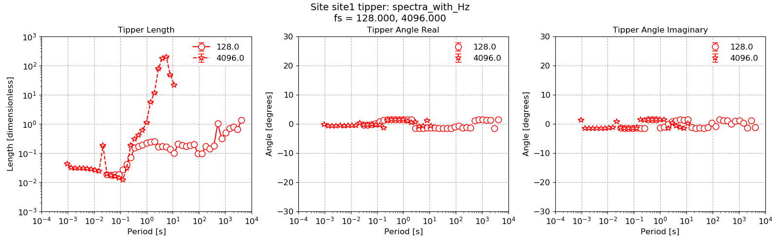
Plot of the tipper result when Hz is added to the output channels
However, including the tipper in the overall calculation may change the estimation of the components of the impedance tensor in the robust regression. The impedance tensor estimate from this process run can be viewed by:
20 21 22 23 24 25 26 27 28 29 30 31 | # plot the transfer function
from resistics.project.transfunc import viewImpedance
figs = viewImpedance(
projData,
sites=["site1"],
polarisations=["ExHy", "EyHx"],
postpend="with_Hz",
save=False,
show=False,
)
figs[0].savefig(imagePath / "simpleRunWithTipper_viewimp_withHz_polarisations")
|
Running with Hz as an output channel produces the below impedance tensor estimate, which is comparable to the one calculated in the previous section.
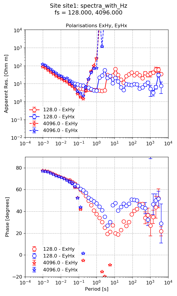
Plot of the impedance tensor result when Hz is added to the output channels
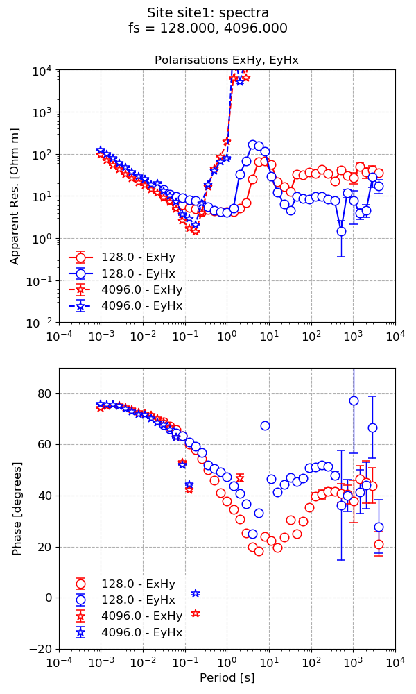
Plot of the impedance tensor result when Hz is excluded from the output channels
As stated earlier, another way to calculate the tipper is to use Hz as the only output channel. An example of how to do this is shown here.
33 34 35 36 | # process only the tippers
processProject(projData, sites=["site1"], outchans=["Hz"], postpend="only_Hz")
figs = viewTipper(projData, sites=["site1"], postpend="only_Hz", save=False, show=False)
figs[0].savefig(imagePath / "simpleRunWithTipper_viewtip_onlyHz")
|
The tipper result is given in the below figure. The result here is different to the result above when Hz is one of a set of output channels.
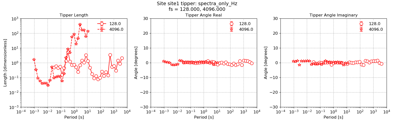
Plot of the tipper result when Hz is set as the only output channel
Complete example script
For the purposes of clarity, the complete example script is provided below.
1 2 3 4 5 6 7 8 9 10 11 12 13 14 15 16 17 18 19 20 21 22 23 24 25 26 27 28 29 30 31 32 33 34 35 36 | from datapaths import projectPath, imagePath
from resistics.project.io import loadProject
# load the project
projData = loadProject(projectPath)
# process the spectra with tippers
from resistics.project.transfunc import processProject
processProject(
projData, sites=["site1"], outchans=["Ex", "Ey", "Hz"], postpend="with_Hz"
)
# plot the tippers
from resistics.project.transfunc import viewTipper

figs = viewTipper(projData, sites=["site1"], postpend="with_Hz", save=True, show=False)
figs[0].savefig(imagePath / "simpleRunWithTipper_viewtip_withHz")
# plot the transfer function
from resistics.project.transfunc import viewImpedance

figs = viewImpedance(
    projData,
    sites=["site1"],
    polarisations=["ExHy", "EyHx"],
    postpend="with_Hz",
    save=False,
    show=False,
)
figs[0].savefig(imagePath / "simpleRunWithTipper_viewimp_withHz_polarisations")
# process only the tippers
processProject(projData, sites=["site1"], outchans=["Hz"], postpend="only_Hz")
figs = viewTipper(projData, sites=["site1"], postpend="only_Hz", save=False, show=False)
figs[0].savefig(imagePath / "simpleRunWithTipper_viewtip_onlyHz")
|