Masks
Statistics give information about individual time windows. In resistics, masks are the way this information can be used.
A mask is used to exclude time windows from the transfer function calculation. Mask data is stored under the maskData folder. Masks are not individual to a specific time series measurement. Instead they are indexed by:
The site
The specdir
The sampling frequency
For example:
exampleProject
├── calData
├── timeData
│   └── site1
|       |── dataFolder1
│       |── dataFolder2
|       |──     .
|       |──     .
|       |──     .
|       └── dataFolderN
├── specData
│   └── site1
|       |── dataFolder1
|       |   |── dec8_5
|       |   └── spectra
|       |
│       |── dataFolder2
|       |   |── dec8_5
|       |   └── spectra
|       |──     .
|       |──     .
|       |──     .
|       └── dataFolderN
|           |── dec8_5
|           └── spectra
├── statData
│   └── site1
|       |── dataFolder1
|       |   |── dec8_5
|       |   |   |── coherence
|       |   |   |──     .
|       |   |   |──     .
|       |   |   |──     .
|       |   |   |── resPhase
|       |   |   └── transferFunction
|       |   └── spectra
|       |       |── coherence
|       |       |──     .
|       |       |──     .
|       |       |──     .
|       |       |── resPhase
|       |       └── transferFunction
|       |
│       |── dataFolder2
|       |   |── dec8_5
|       |   |   |── coherence
|       |   |   |──     .
|       |   |   |──     .
|       |   |   |──     .
|       |   |   |── resPhase
|       |   |   └── transferFunction
|       |   └── spectra
|       |       |── coherence
|       |       |──     .
|       |       |──     .
|       |       |──     .
|       |       |── resPhase
|       |       └── transferFunction
|       |──     .
|       |──     .
|       |──     .
|       └── dataFolderN
|           |── dec8_5
|           |   |── coherence
|           |   |──     .
|           |   |──     .
|           |   |──     .
|           |   |── resPhase
|           |   └── transferFunction
|           └── spectra
|               |── coherence
|               |──     .
|               |──     .
|               |──     .
|               |── resPhase
|               └── transferFunction
├── maskData
│   └── site1
|       └── dec8_5
|           |── {coh70_100_128_000.npy, coh70_100_128_000.info}
|           └── {coh70_100_4096_000.npy, coh70_100_4096_000.info}
├── transFuncData
├── images
└── mtProj.prj
Mask data is made up of two files:
The info file: coh70_100_128_000.info
The mask data file: coh70_100_128_000.npy
The info file holds information about the statistics and constraints used to generate the mask file. The mask data is simply numpy array data holding information about which time windows to exclude.
The easiest way to understand masking is to step through an example. Begin, as usual, by loading the project.
1 2 3 4 5 | from datapaths import projectPath, imagePath
from resistics.project.io import loadProject
# load project and configuration file
projData = loadProject(projectPath, configFile="tutorialConfig.ini")
|
To generate new mask data, the method newMaskData() in project module mask is used. To create a new mask, the sampling frequency to which the mask applies must be specified.
7 8 9 10 | # get a mask data object and specify the sampling frequency to mask (128Hz)
from resistics.project.mask import newMaskData
maskData = newMaskData(projData, 128)
|
The method newMaskData() returns a MaskData object, which will hold information about the statistics to use and the constraints.
The next step is to set the statistics to use for excluding windows. These statistics must already be calculated and were so in the Statistics section.
11 12 | # set the statistics to use in our masking - these must already be calculated out
maskData.setStats(["coherence"])
|
After the statistics are chosen, the constraints can be defined.
13 14 | # window must have the coherence parameters "cohExHy" and "cohEyHx" both between 0.7 and 1.0
maskData.addConstraint("coherence", {"cohExHy": [0.7, 1.0], "cohEyHx": [0.7, 1.0]})
|
In the above example, a mask is being created that requires the Ex-Hy coherence and the Ey-Hx coherence to be between 0.70 and 1.00 for a time window. If this is not the case, then the time window will be masked (excluded) for the transfer funciton calculation.
Before writing out a mask dataset, the MaskData instance should be given a name.
15 16 | # give maskData a name, which will relate to the output file
maskData.maskName = "coh70_100"
|
The naming of mask files is made up of two parts:
The mask name
The sampling frequency written to 3 decimal places and using a _ rather than . to indicate the decimal point (i.e. 128.000 becomes 128_000)
Therefore, for the above example, the mask files will be:
The info file: coh70_100_128_000.info
The mask data file: coh70_100_128_000.npy
The MaskData parameters can be viewed by using the printInfo() method of the ResisticsBase parent class. The masking constraints can be printed to the terminal using the printConstraints() method.
17 18 19 | # print info to see what has been added
maskData.printInfo()
maskData.printConstraints()
|
So far, the following information has been defined:
The sampling frequency
The statistics to use for masking
The constraints for the statistics
However, the windows to mask have not yet been calculated. This is achieved by using the calculateMask() method of the project module mask. This method runs through the pre-calculated statistic data for all data of the given sampling frequency in a site and finds and saves the windows which do not meet the constraints.
21 22 23 24 25 26 | # calculate a file of masked windows for the sampling frequency associated with the maskData
from resistics.project.mask import calculateMask
calculateMask(projData, maskData, sites=["site1"])
fig = maskData.view(0)
fig.savefig(imagePath / "usingMasks_maskData_128_coh_dec0")
|
As statistics are calculated on an evaluation frequency basis, masked windows are calculated for each evaluation frequency too.
Once the masked windows are calculated, they can then be viewed using the view() method of MaskData. When using the view() method, the decimation level has to be specified. In the example above, this has been set to 0, which is the first decimation level. The resultant plot is shown below.
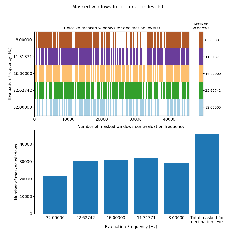
Mask data plot for 128 Hz data using coherence constraints of 0.70-1.00
The bar chart at the bottom shows the number of masked windows for each evaluation frequency in the decimation level, plus the total number of masked windows for the decimation level. The top plot shows all the masked windows for the decimation level and which ones of those are masked for the individual evaluation frequencies. Poor quality time windows will generally be masked across all the evaluation frequencies.
The same process can be repeated for the 4096 Hz data.
28 29 30 31 32 33 34 35 36 37 | # do the same for 4096 Hz
maskData = newMaskData(projData, 4096)
maskData.setStats(["coherence"])
maskData.addConstraint("coherence", {"cohExHy": [0.7, 1.0], "cohEyHx": [0.7, 1.0]})
maskData.maskName = "coh70_100"
maskData.printInfo()
maskData.printConstraints()
calculateMask(projData, maskData, sites=["site1"])
fig = maskData.view(0)
fig.savefig(imagePath / "usingMasks_maskData_4096_coh_dec0")
|
The mask data plot for the 4096 Hz data is shown below.
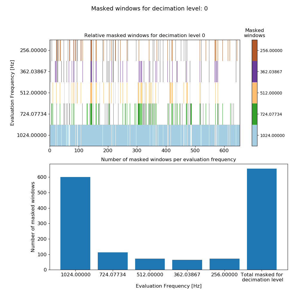
Mask data plot for 4096 Hz data using coherence constraints of 0.70-1.00
Calculating masks with more than a single statistic can be done too. However, it is important to remember that only time windows which satisfy all the constraints will be used in the transfer function calculation. In the below example, a new mask is calculated using two statistics, coherence and transfer function.
39 40 41 42 43 44 45 46 47 48 49 50 51 52 53 54 55 | # calculate out statistics again, but this time use both transfer function and coherence
maskData = newMaskData(projData, 128)
maskData.setStats(["coherence", "transferFunction"])
maskData.addConstraint("coherence", {"cohExHy": [0.7, 1.0], "cohEyHx": [0.7, 1.0]})
maskData.addConstraint(
"transferFunction",
{
"ExHyReal": [-500, 500],
"ExHyImag": [-500, 500],
"EyHxReal": [-500, 500],
"EyHxImag": [-500, 500],
},
)
maskData.maskName = "coh70_100_tfConstrained"
calculateMask(projData, maskData, sites=["site1"])
fig = maskData.view(0)
fig.savefig(imagePath / "usingMasks_maskData_128_coh_tf_dec0")
|
This produces the plot:
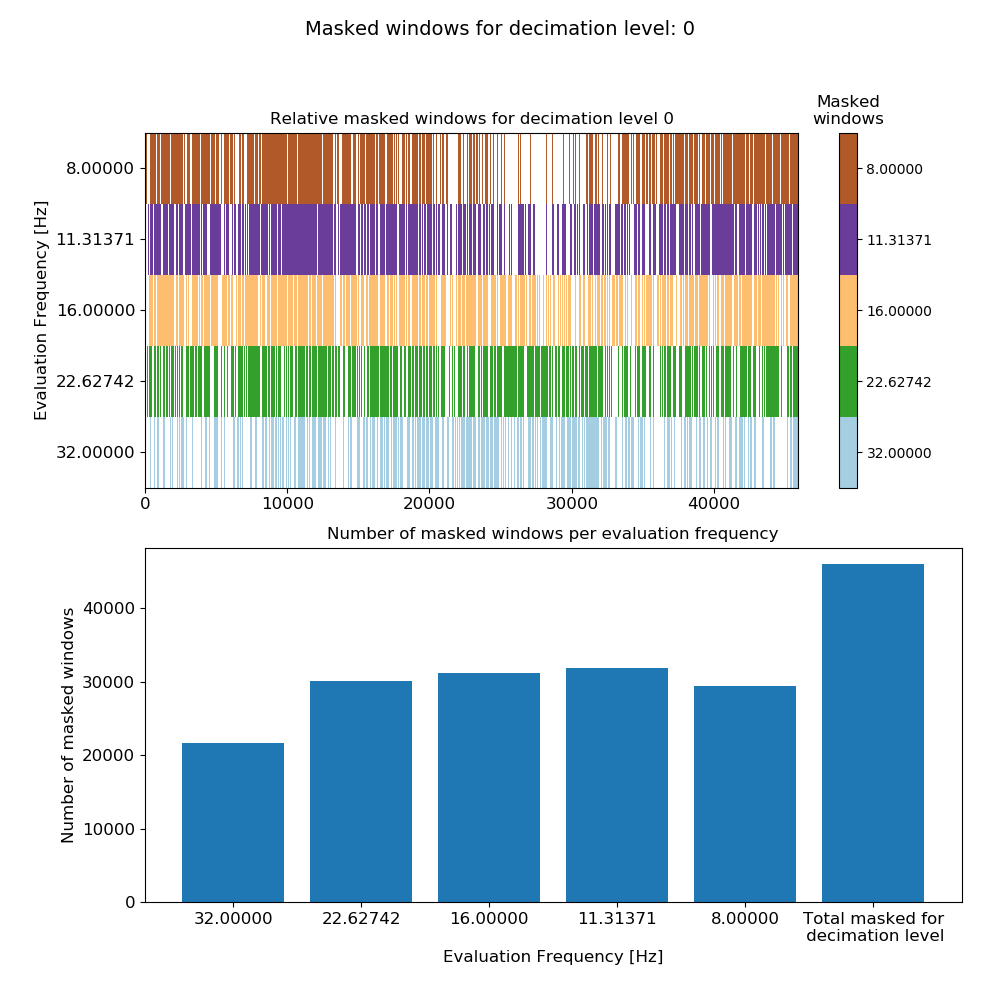
Mask data plot for 128 Hz data using coherence constraints of 0.70-1.00 and constraints on the transfer function values calculated on an individual window basis.
Notice that adding more constraints has increased the number of masked windows as expected. Repeating the exercise with the 4096 Hz data:
57 58 59 60 61 62 63 64 65 66 67 68 69 70 71 72 | maskData = newMaskData(projData, 4096)
maskData.setStats(["coherence", "transferFunction"])
maskData.addConstraint("coherence", {"cohExHy": [0.7, 1.0], "cohEyHx": [0.7, 1.0]})
maskData.addConstraint(
"transferFunction",
{
"ExHyReal": [-500, 500],
"ExHyImag": [-500, 500],
"EyHxReal": [-500, 500],
"EyHxImag": [-500, 500],
},
)
maskData.maskName = "coh70_100_tfConstrained"
calculateMask(projData, maskData, sites=["site1"])
fig = maskData.view(0)
fig.savefig(imagePath / "usingMasks_maskData_4096_coh_tf_dec0")
|
This produces the plot:
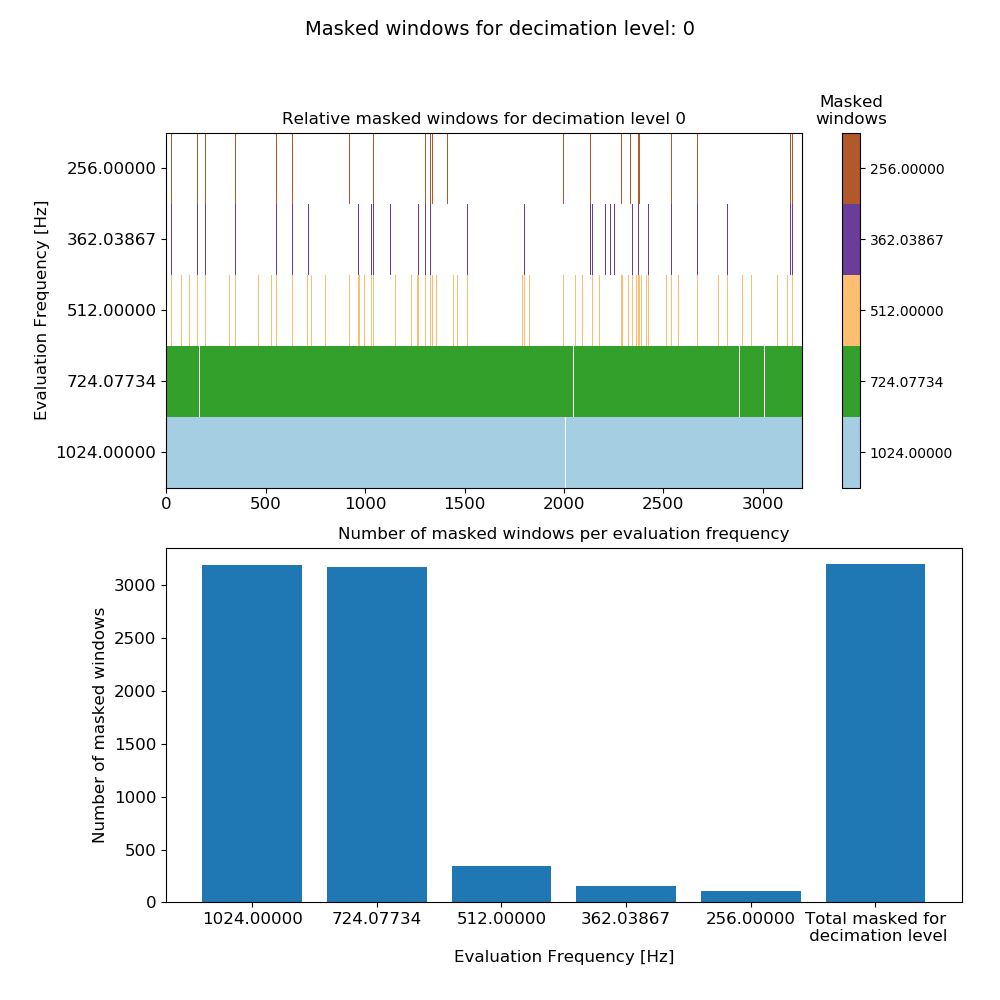
Mask data plot for 4096 Hz data using coherence constraints of 0.70-1.00 and constraints on the transfer function values calculated on an individual window basis.
Here, the constraints have masked many windows for evaluation frequencies 1024 Hz and 724.077344 Hz. This is almost certainly over-zealous for these two evaluation frequencies (but to better understand how over-zealous read further down).
Up until now, all mask constraints have been specified globally (i.e. as applying to all evaluation frequencies). However, statistic constraints can be defined in a more targeted manner, at evaluation frequencies that are noisier than others. More targeted constraints can be specified using the listed methods.
addConstraintLevel()method ofMaskData, which allows setting constraints just for a specific decimation level.addConstraintFreq()method ofMaskData, which allows setting constraints for a specific evaluation frequency.
Using the second option requires specification of decimation level and evaluation frequency. In resistics, these are generally specified using indices as shown in the Statistics section.
Important
It is worth repeating here the meaning of the decimation level index and evaluation frequency index, which was previously covered in Statistics.
Consider the evaluation frequencies in this set up using 8 decimation levels and 5 evaluation frequencies per level with a data sampling frequency of 128 Hz:
Decimation Level = 0: 32.00000000, 22.62741700, 16.00000000, 11.31370850, 8.00000000 Decimation Level = 1: 5.65685425, 4.00000000, 2.82842712, 2.00000000, 1.41421356 Decimation Level = 2: 1.00000000, 0.70710678, 0.50000000, 0.35355339, 0.25000000 Decimation Level = 3: 0.17677670, 0.12500000, 0.08838835, 0.06250000, 0.04419417 Decimation Level = 4: 0.03125000, 0.02209709, 0.01562500, 0.01104854, 0.00781250 Decimation Level = 5: 0.00552427, 0.00390625, 0.00276214, 0.00195312, 0.00138107 Decimation Level = 6: 0.00097656, 0.00069053, 0.00048828, 0.00034527, 0.00024414 Decimation Level = 7: 0.00017263, 0.00012207, 0.00008632, 0.00006104, 0.00004316Decimation level numbering starts from 0 (and with 8 decimation levels, extends to 7). Evaluation frequency numbering begins from 0 (and with 5 evaluation frequencies per decimation level, extends to 4).
The decimation and evaluation frequency indices can be best demonstrated using a few of examples:
Evaluation frequency 32 Hz, decimation level = 0, evaluation frequency index = 0
Evaluation frequency 1 Hz, decimation level = 2, evaluation frequency index = 0
Evaluation frequency 0.35355339 Hz, decimation level = 2, evaluation frequency index = 3
The main motivation behind this is the difficulty in manually specifying evaluation frequencies such as 0.35355339 Hz.
The impact of masks on statistics
A more useful visualisation of masks is to see how removing selected time windows effects the statistics. In the Statistics section, the plotting of statistics was demonstrated. Plotting statistics with masks applied is similar.
Load the project and use the getMaskData() method of the mask module to open up a previous calculated mask dataset at a sampling frequency of 4096 Hz.
1 2 3 4 5 6 7 8 9 10 | from datapaths import projectPath, imagePath
from resistics.project.io import loadProject
# load project and configuration file
projData = loadProject(projectPath, configFile="tutorialConfig.ini")
# get mask data
from resistics.project.mask import getMaskData
maskData = getMaskData(projData, "site1", "coh70_100", 4096)
|
Next, get a set of masked windows for an evaluation frequency of 1024 Hz, which translates to decimation level 0 and evaluation frequency index 0.
11 12 | # get the masked windows for decimation level 0 and evaluation frequency index 0
maskWindows = maskData.getMaskWindowsFreq(0, 0)
|
To be able to plot the statistic data, this needs to be loaded too and can be by using the getStatisticData() method of project module statistics. For more information, see the Statistics section.
14 15 16 17 18 19 | # get statistic data
from resistics.project.statistics import getStatisticData
statData = getStatisticData(
projData, "site1", "meas_2012-02-10_11-05-00", "transferFunction"
)
|
Now the statistic data can be plotted with the mask data. In the examples below, the statistic data is plotted both with and without masking to demonstrate the difference.
Viewing transfer function statistic data:
21 22 23 24 25 | # view masked statistic data again but this with constraints on both coherence and transfer function
fig = statData.view(0, ylim=[-2000, 2000])
fig.savefig(imagePath / "masksAndStats_statistic_4096_nomask_view")
fig = statData.view(0, maskwindows=maskWindows, ylim=[-2000, 2000])
fig.savefig(imagePath / "masksAndStats_statistic_4096_maskcoh_view")
|
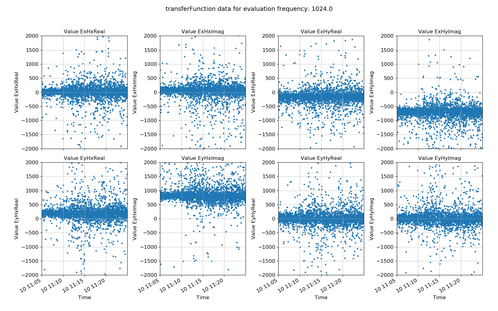
Transfer function statistic data without masking
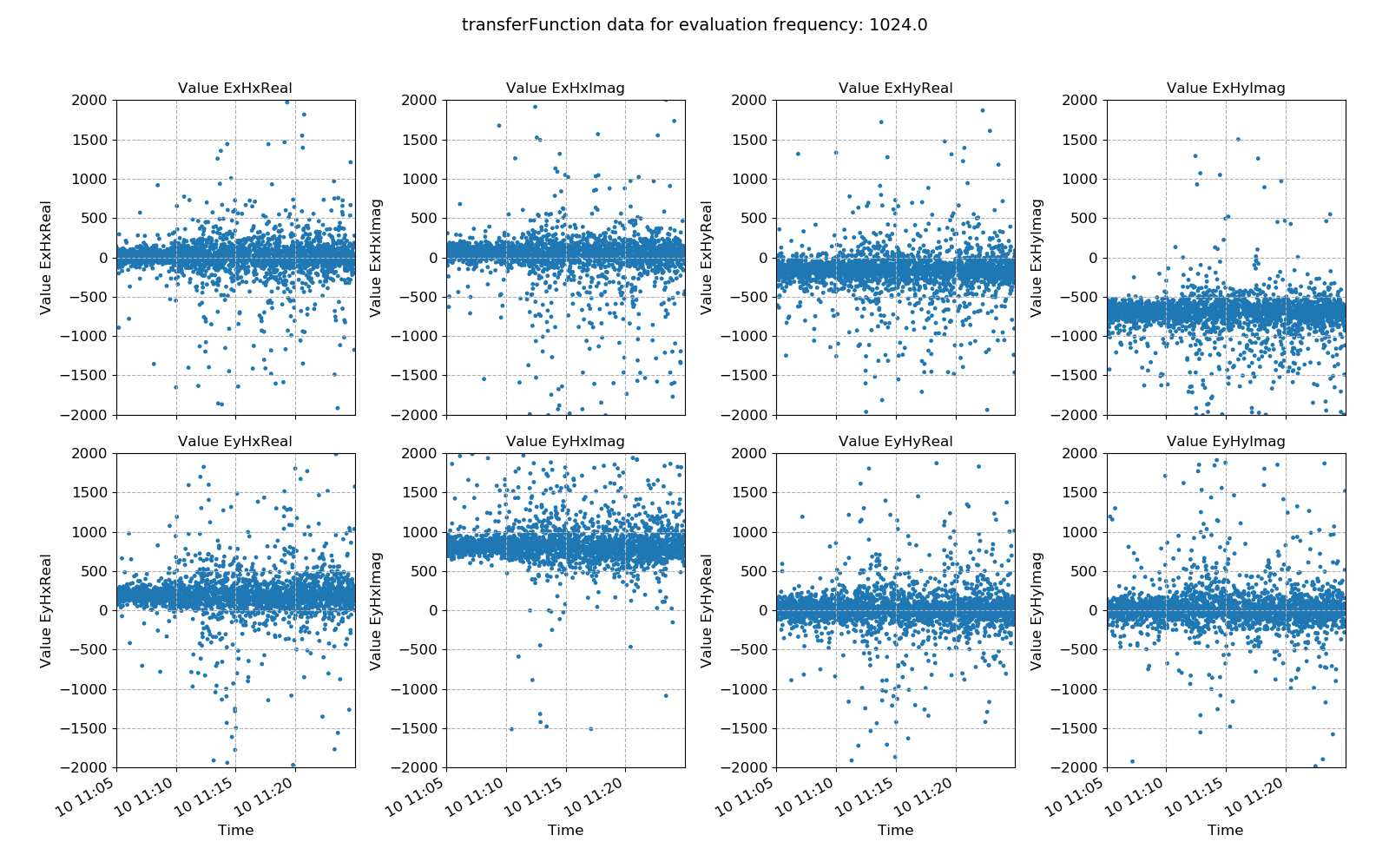
Transfer function statistic data with masking (constraints on only coherence)
Ideally, the effect of masking should lead to more consistency in the various components of the transfer function, with less scatter. In this case, coherence based time window masking has reduced the scatter around the average value, which will lead to an improvement in the robust regression for transfer funciton estimation.
Histograms of transfer function statistic data:
26 27 28 29 30 | # histogram
fig = statData.histogram(0, xlim=[-1000, 1000])
fig.savefig(imagePath / "masksAndStats_statistic_4096_nomask_hist")
fig = statData.histogram(0, maskwindows=maskWindows, xlim=[-1000, 1000])
fig.savefig(imagePath / "masksAndStats_statistic_4096_maskcoh_hist")
|
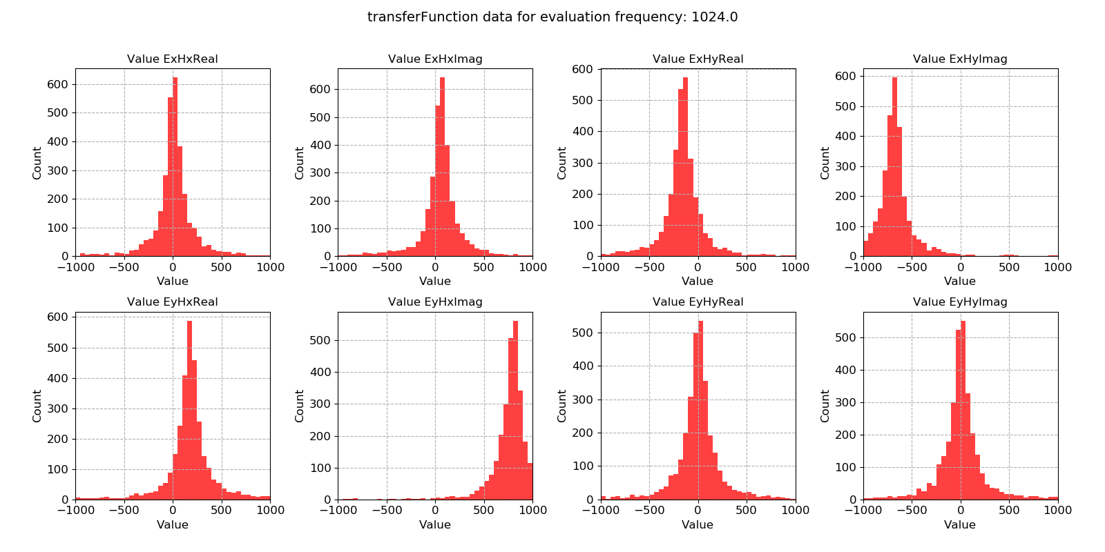
Transfer function statistic histogram without masking
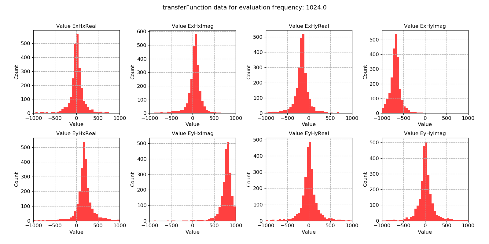
Transfer function statistic histogram with masking (constraints on only coherence)
For the transfer function statistic, Gaussian distributions across the windows is an indication that the overall transfer function estimate will be good. In situations where window-by-window transfer function estimates are not near Gaussian distributed, the resultant overall transfer function estimation will normally be poor. Here, the data is quite well distributed.
Crossplots of transfer function statistic data:
31 32 33 34 35 36 37 38 39 40 41 42 43 44 45 46 47 48 49 50 51 52 53 54 55 56 | # crossplot
fig = statData.crossplot(
0,
crossplots=[
["ExHxReal", "ExHxImag"],
["ExHyReal", "ExHyImag"],
["EyHxReal", "EyHxImag"],
["EyHyReal", "EyHyImag"],
],
xlim=[-2500, 2500],
ylim=[-2500, 2500],
)
fig.savefig(imagePath / "masksAndStats_statistic_4096_nomask_crossplot")
fig = statData.crossplot(
0,
maskwindows=maskWindows,
crossplots=[
["ExHxReal", "ExHxImag"],
["ExHyReal", "ExHyImag"],
["EyHxReal", "EyHxImag"],
["EyHyReal", "EyHyImag"],
],
xlim=[-2500, 2500],
ylim=[-2500, 2500],
)
fig.savefig(imagePath / "masksAndStats_statistic_4096_maskcoh_crossplot")
|
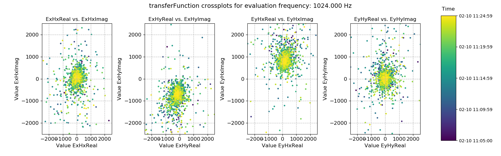
Transfer function statistic crossplot without masking
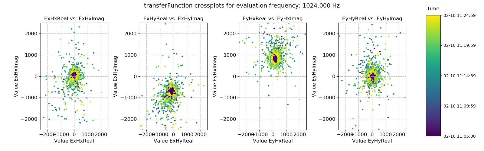
Transfer function statistic crossplot with masking (constraints on only coherence)
Plotting the window-by-window transfer function estimation in the complex plane should ideally yield a tight scatter of points around an average point. Where this is not the case, the overall transfer function estimate will tend to be poor. In this case, the data is good.
Repeating the same process with the second mask that was calculated (using both coherence and transfer function constraints) is easily done.
58 59 60 61 62 63 64 65 66 67 68 69 70 71 72 73 74 75 76 77 | # view statistic data again but this time exclude the masked windows
maskData = getMaskData(projData, "site1", "coh70_100_tfConstrained", 4096)
maskWindows = maskData.getMaskWindowsFreq(0, 0)
fig = statData.view(0, maskwindows=maskWindows, ylim=[-2000, 2000])
fig.savefig(imagePath / "masksAndStats_statistic_4096_maskcoh_tf_view")
fig = statData.histogram(0, maskwindows=maskWindows, xlim=[-1000, 1000])
fig.savefig(imagePath / "masksAndStats_statistic_4096_maskcoh_tf_hist")
fig = statData.crossplot(
0,
maskwindows=maskWindows,
crossplots=[
["ExHxReal", "ExHxImag"],
["ExHyReal", "ExHyImag"],
["EyHxReal", "EyHxImag"],
["EyHyReal", "EyHyImag"],
],
xlim=[-2500, 2500],
ylim=[-2500, 2500],
)
fig.savefig(imagePath / "masksAndStats_statistic_4096_maskcoh_tf_crossplot")
|
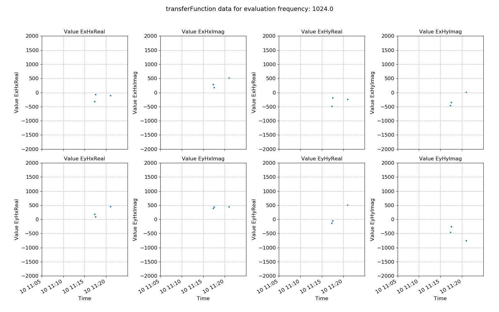
Transfer function statistic with masking (constraints on both coherence and transfer function)
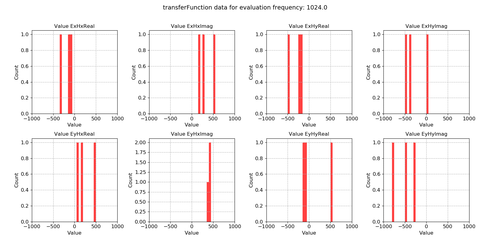
Transfer function statistic histogram with masking (constraints on both coherence and transfer function)
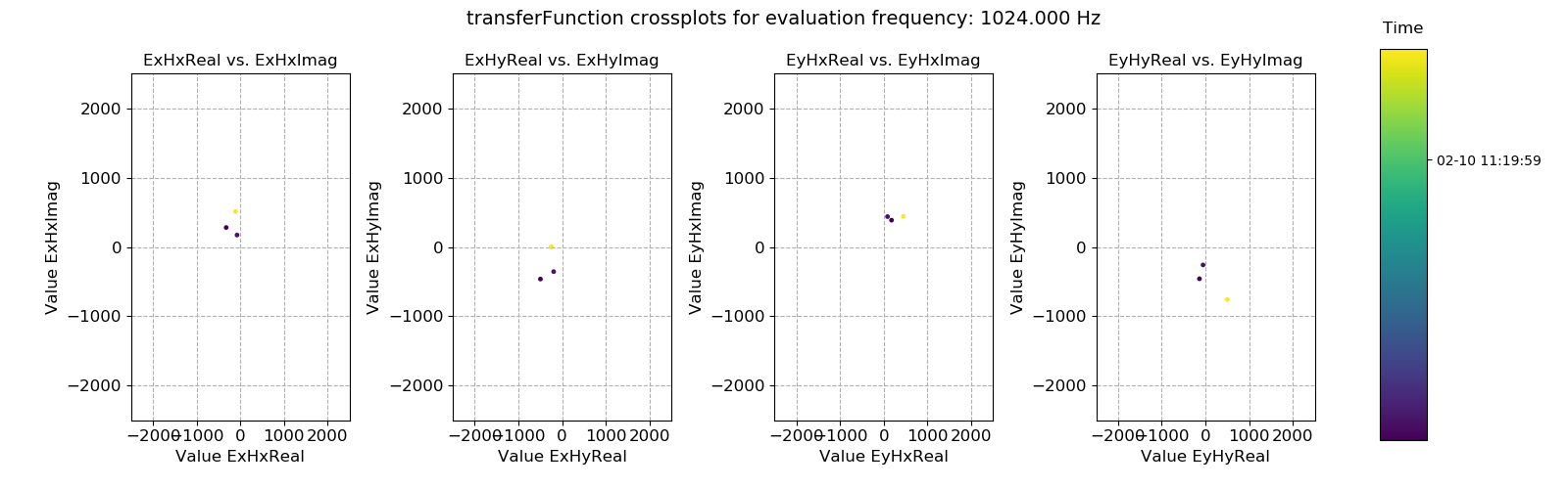
Transfer function statistic crossplot with masking (constraints on both coherence and transfer function)
As suggested earlier, adding the extra mask constraints for this evaluation frequency was over-zealous, mainly due to the ExHyImag and EyHxImag constraints. Only a handful of time windows meet these constraints and the transfer function estimate at this evaluation frequency is likely to be poorer than when simply using the coherence mask.
Remember that statistic data is saved for each individual time series measurement directory. Hence, currently only the statistic values from one time series recordings are being considered. To really understand how masking windows will influence the transfer function calculation, the effect on the statistics for all time series measurements at a single sampling frequency in a site needs to be considered. This information can be plotted using the viewStatistic() and viewStatisticHistogram() of the project statistics module. An example is provided below.
79 80 81 82 83 84 85 86 87 88 89 90 91 92 93 94 95 96 97 98 99 100 101 102 103 104 105 106 107 108 | # if there are more than one data folder for the same site at the same sampling frequency
# the better way to plot statistics with masks is using the methods in projectStatistics
from resistics.project.statistics import viewStatistic, viewStatisticHistogram
from resistics.common.plot import plotOptionsStandard, getPaperFonts
plotOptions = plotOptionsStandard(plotfonts=getPaperFonts())
fig = viewStatistic(
projData,
"site1",
128,
"coherence",
maskname="coh70_100",
ylim=[0, 1],
save=False,
show=False,
plotoptions=plotOptions,
)
fig.savefig(imagePath / "masksAndStats_projstat_128_maskcoh_coh_view")
viewStatisticHistogram(
projData,
"site1",
128,
"coherence",
maskname="coh70_100",
xlim=[0, 1],
save=False,
show=False,
plotoptions=plotOptions,
)
fig.savefig(imagePath / "masksAndStats_projstat_128_maskcoh_coh_hist")
|
Warning
These plots can be quite intensive due to the number of time windows in the data. Therefore, it is usually best to save them rather than show them.
The result plots are shown below.
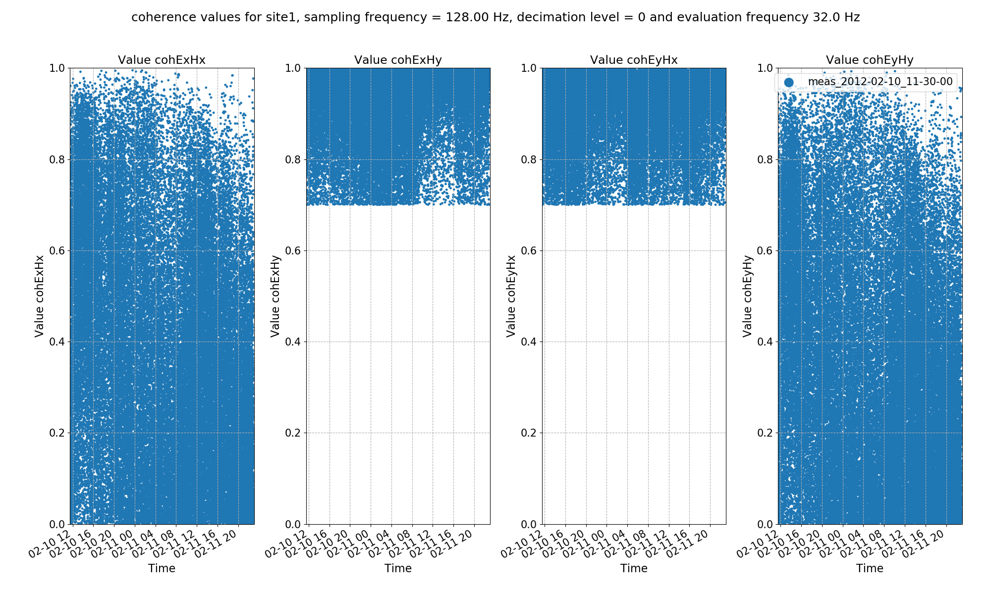
Transfer function statistic histogram with masking (constraints on both coherence and transfer function)

Transfer function statistic crossplot with masking (constraints on both coherence and transfer function)
Now that masks have been calculated, the next stage is to use the masks in the transfer function estimation, which is demonstrated in the Processing with masks section.
Complete example script
For the purposes of clarity, the complete example scripts are provided below.
For calculating masks from statistics:
1 2 3 4 5 6 7 8 9 10 11 12 13 14 15 16 17 18 19 20 21 22 23 24 25 26 27 28 29 30 31 32 33 34 35 36 37 38 39 40 41 42 43 44 45 46 47 48 49 50 51 52 53 54 55 56 57 58 59 60 61 62 63 64 65 66 67 68 69 70 71 72 73 | from datapaths import projectPath, imagePath
from resistics.project.io import loadProject
# load project and configuration file
projData = loadProject(projectPath, configFile="tutorialConfig.ini")
# get a mask data object and specify the sampling frequency to mask (128Hz)
from resistics.project.mask import newMaskData

maskData = newMaskData(projData, 128)
# set the statistics to use in our masking - these must already be calculated out
maskData.setStats(["coherence"])
# window must have the coherence parameters "cohExHy" and "cohEyHx" both between 0.7 and 1.0
maskData.addConstraint("coherence", {"cohExHy": [0.7, 1.0], "cohEyHx": [0.7, 1.0]})
# give maskData a name, which will relate to the output file
maskData.maskName = "coh70_100"
# print info to see what has been added
maskData.printInfo()
maskData.printConstraints()
# calculate a file of masked windows for the sampling frequency associated with the maskData
from resistics.project.mask import calculateMask

calculateMask(projData, maskData, sites=["site1"])
fig = maskData.view(0)
fig.savefig(imagePath / "usingMasks_maskData_128_coh_dec0")
# do the same for 4096 Hz
maskData = newMaskData(projData, 4096)
maskData.setStats(["coherence"])
maskData.addConstraint("coherence", {"cohExHy": [0.7, 1.0], "cohEyHx": [0.7, 1.0]})
maskData.maskName = "coh70_100"
maskData.printInfo()
maskData.printConstraints()
calculateMask(projData, maskData, sites=["site1"])
fig = maskData.view(0)
fig.savefig(imagePath / "usingMasks_maskData_4096_coh_dec0")
# calculate out statistics again, but this time use both transfer function and coherence
maskData = newMaskData(projData, 128)
maskData.setStats(["coherence", "transferFunction"])
maskData.addConstraint("coherence", {"cohExHy": [0.7, 1.0], "cohEyHx": [0.7, 1.0]})
maskData.addConstraint(
    "transferFunction",
    {
        "ExHyReal": [-500, 500],
        "ExHyImag": [-500, 500],
        "EyHxReal": [-500, 500],
        "EyHxImag": [-500, 500],
    },
)
maskData.maskName = "coh70_100_tfConstrained"
calculateMask(projData, maskData, sites=["site1"])
fig = maskData.view(0)
fig.savefig(imagePath / "usingMasks_maskData_128_coh_tf_dec0")
maskData = newMaskData(projData, 4096)
maskData.setStats(["coherence", "transferFunction"])
maskData.addConstraint("coherence", {"cohExHy": [0.7, 1.0], "cohEyHx": [0.7, 1.0]})
maskData.addConstraint(
    "transferFunction",
    {
        "ExHyReal": [-500, 500],
        "ExHyImag": [-500, 500],
        "EyHxReal": [-500, 500],
        "EyHxImag": [-500, 500],
    },
)
maskData.maskName = "coh70_100_tfConstrained"
calculateMask(projData, maskData, sites=["site1"])
fig = maskData.view(0)
fig.savefig(imagePath / "usingMasks_maskData_4096_coh_tf_dec0")
|
To see the impact of masks on statistics:
1 2 3 4 5 6 7 8 9 10 11 12 13 14 15 16 17 18 19 20 21 22 23 24 25 26 27 28 29 30 31 32 33 34 35 36 37 38 39 40 41 42 43 44 45 46 47 48 49 50 51 52 53 54 55 56 57 58 59 60 61 62 63 64 65 66 67 68 69 70 71 72 73 74 75 76 77 78 79 80 81 82 83 84 85 86 87 88 89 90 91 92 93 94 95 96 97 98 99 100 101 102 103 104 105 106 107 108 | from datapaths import projectPath, imagePath
from resistics.project.io import loadProject
# load project and configuration file
projData = loadProject(projectPath, configFile="tutorialConfig.ini")
# get mask data
from resistics.project.mask import getMaskData
maskData = getMaskData(projData, "site1", "coh70_100", 4096)
# get the masked windows for decimation level 0 and evaluation frequency index 0
maskWindows = maskData.getMaskWindowsFreq(0, 0)
# get statistic data
from resistics.project.statistics import getStatisticData

statData = getStatisticData(
    projData, "site1", "meas_2012-02-10_11-05-00", "transferFunction"
)
# view masked statistic data again but this with constraints on both coherence and transfer function
fig = statData.view(0, ylim=[-2000, 2000])
fig.savefig(imagePath / "masksAndStats_statistic_4096_nomask_view")
fig = statData.view(0, maskwindows=maskWindows, ylim=[-2000, 2000])
fig.savefig(imagePath / "masksAndStats_statistic_4096_maskcoh_view")
# histogram
fig = statData.histogram(0, xlim=[-1000, 1000])
fig.savefig(imagePath / "masksAndStats_statistic_4096_nomask_hist")
fig = statData.histogram(0, maskwindows=maskWindows, xlim=[-1000, 1000])
fig.savefig(imagePath / "masksAndStats_statistic_4096_maskcoh_hist")
# crossplot
fig = statData.crossplot(
    0,
    crossplots=[
        ["ExHxReal", "ExHxImag"],
        ["ExHyReal", "ExHyImag"],
        ["EyHxReal", "EyHxImag"],
        ["EyHyReal", "EyHyImag"],
    ],
    xlim=[-2500, 2500],
    ylim=[-2500, 2500],
)
fig.savefig(imagePath / "masksAndStats_statistic_4096_nomask_crossplot")
fig = statData.crossplot(
    0,
    maskwindows=maskWindows,
    crossplots=[
        ["ExHxReal", "ExHxImag"],
        ["ExHyReal", "ExHyImag"],
        ["EyHxReal", "EyHxImag"],
        ["EyHyReal", "EyHyImag"],
    ],
    xlim=[-2500, 2500],
    ylim=[-2500, 2500],
)
fig.savefig(imagePath / "masksAndStats_statistic_4096_maskcoh_crossplot")
# view statistic data again but this time exclude the masked windows
maskData = getMaskData(projData, "site1", "coh70_100_tfConstrained", 4096)
maskWindows = maskData.getMaskWindowsFreq(0, 0)
fig = statData.view(0, maskwindows=maskWindows, ylim=[-2000, 2000])
fig.savefig(imagePath / "masksAndStats_statistic_4096_maskcoh_tf_view")
fig = statData.histogram(0, maskwindows=maskWindows, xlim=[-1000, 1000])
fig.savefig(imagePath / "masksAndStats_statistic_4096_maskcoh_tf_hist")
fig = statData.crossplot(
    0,
    maskwindows=maskWindows,
    crossplots=[
        ["ExHxReal", "ExHxImag"],
        ["ExHyReal", "ExHyImag"],
        ["EyHxReal", "EyHxImag"],
        ["EyHyReal", "EyHyImag"],
    ],
    xlim=[-2500, 2500],
    ylim=[-2500, 2500],
)
fig.savefig(imagePath / "masksAndStats_statistic_4096_maskcoh_tf_crossplot")
# if there are more than one data folder for the same site at the same sampling frequency
# the better way to plot statistics with masks is using the methods in projectStatistics
from resistics.project.statistics import viewStatistic, viewStatisticHistogram
from resistics.common.plot import plotOptionsStandard, getPaperFonts

plotOptions = plotOptionsStandard(plotfonts=getPaperFonts())
fig = viewStatistic(
    projData,
    "site1",
    128,
    "coherence",
    maskname="coh70_100",
    ylim=[0, 1],
    save=False,
    show=False,
    plotoptions=plotOptions,
)
fig.savefig(imagePath / "masksAndStats_projstat_128_maskcoh_coh_view")
viewStatisticHistogram(
    projData,
    "site1",
    128,
    "coherence",
    maskname="coh70_100",
    xlim=[0, 1],
    save=False,
    show=False,
    plotoptions=plotOptions,
)
fig.savefig(imagePath / "masksAndStats_projstat_128_maskcoh_coh_hist")
|