Remote reference statistics
Remote reference statistics are a means of understanding how adding a remote reference site to the processing of magnetotelluric data is changing the solution. There are currently five remote reference statistics.
“RR_coherence”
“RR_coherenceEqn”
“RR_absvalEqn”
“RR_transferFunction”
“RR_resPhase”
More information on each of these is given in remote reference statistics.
Important
Remote reference statistics are always saved with the local site.
Calculating and viewing remote reference statistics
Begin by loading the project and calculate the remote statistics using the calculateRemoteStatistics() of module statistics. The calculateRemoteStatistics() method will calculate the remote reference statistics for sites=[“M6”] and at sampling frequencies sampleFreqs=[128] using the remote site “Remote”. In this instance, all the remote statistics are being calculated.
1 2 3 4 5 6 7 8 9 10 11 12 13 14 15 16 17 18 19 20 21 22 23 24 25 26 27 28 | from datapaths import remotePath, remoteImages
from resistics.project.io import loadProject
from resistics.project.statistics import (
calculateRemoteStatistics,
viewStatistic,
viewStatisticHistogram,
viewStatisticDensityplot,
)
from resistics.project.mask import newMaskData, calculateMask
from resistics.project.transfunc import processProject, viewImpedance
from resistics.common.plot import plotOptionsStandard, getPaperFonts
plotOptions = plotOptionsStandard(plotfonts=getPaperFonts())
proj = loadProject(remotePath)
calculateRemoteStatistics(
proj,
"Remote",
sites=["M6"],
sampleFreqs=[128],
remotestats=[
"RR_coherence",
"RR_coherenceEqn",
"RR_absvalEqn",
"RR_transferFunction",
"RR_resPhase",
],
)
|
To get an idea how the remote reference is changing the impedance tensor values, the impedance tensor estimates for each window for the single site and remote reference processing can now be plotted. To do this, the viewStatisticDensityplot() of module statistics is used. This method plots 2-D histograms of statistic data cross pairs. In the following code snippet, density plots are being saved for the first evaluation frequency of decimation levels 0, 1, 2 and 3. Limits for x and y axes are also being set explicitly.
30 31 32 33 34 35 36 37 38 39 40 41 42 43 44 45 46 47 48 49 50 51 52 53 54 55 56 57 | lims = {0: 200, 1: 120, 2: 50, 3: 30}
for declevel in range(0, 4):
fig = viewStatisticDensityplot(
proj,
"M6",
128,
"RR_transferFunction",
declevel=declevel,
crossplots=[["ExHyRealRR", "ExHyImagRR"], ["EyHxRealRR", "EyHxImagRR"]],
xlim=[-lims[declevel], lims[declevel]],
ylim=[-lims[declevel], lims[declevel]],
plotoptions=plotOptions,
show=False,
)
fig.savefig(remoteImages / "densityPlot_remoteRef_{}.png".format(declevel))
fig = viewStatisticDensityplot(
proj,
"M6",
128,
"transferFunction",
declevel=declevel,
crossplots=[["ExHyReal", "ExHyImag"], ["EyHxReal", "EyHxImag"]],
xlim=[-lims[declevel], lims[declevel]],
ylim=[-lims[declevel], lims[declevel]],
plotoptions=plotOptions,
show=False,
)
fig.savefig(remoteImages / "densityPlot_singleSite_{}.png".format(declevel))
|
For single site statistics, the window-by-window impedance tensor estimates are calculated in the “transferFunction” statistic. This has components: ExHxReal, ExHxImag, ExHyReal, ExHyImag, EyHxReal, EyHxImag, EyHyReal, EyHyImag. For the density plot, the cross pairs ExHyReal vs. ExHyImag and EyHxReal vs. EyHxImag are plotted. This is essentially the Ex-Hy and Ey-Hx polarisations of the single site impedance tensor estimates plotted in the complex plane.
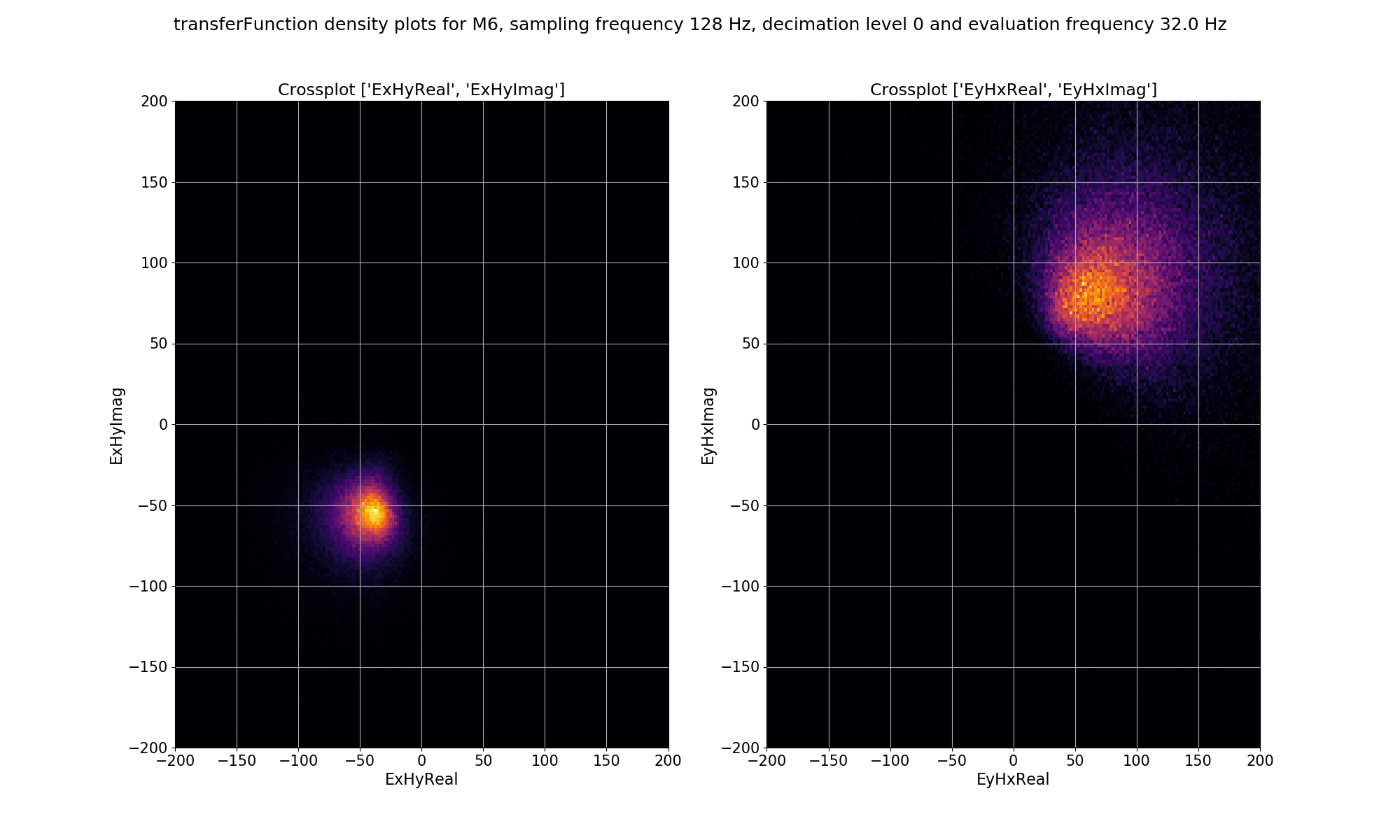
Density plot of single site, window-by-window, impedance tensor Ex-Hy and Ey-Hx estimates for decimation level 0, evaluation frequency 32 Hz or period 0.03125 seconds.
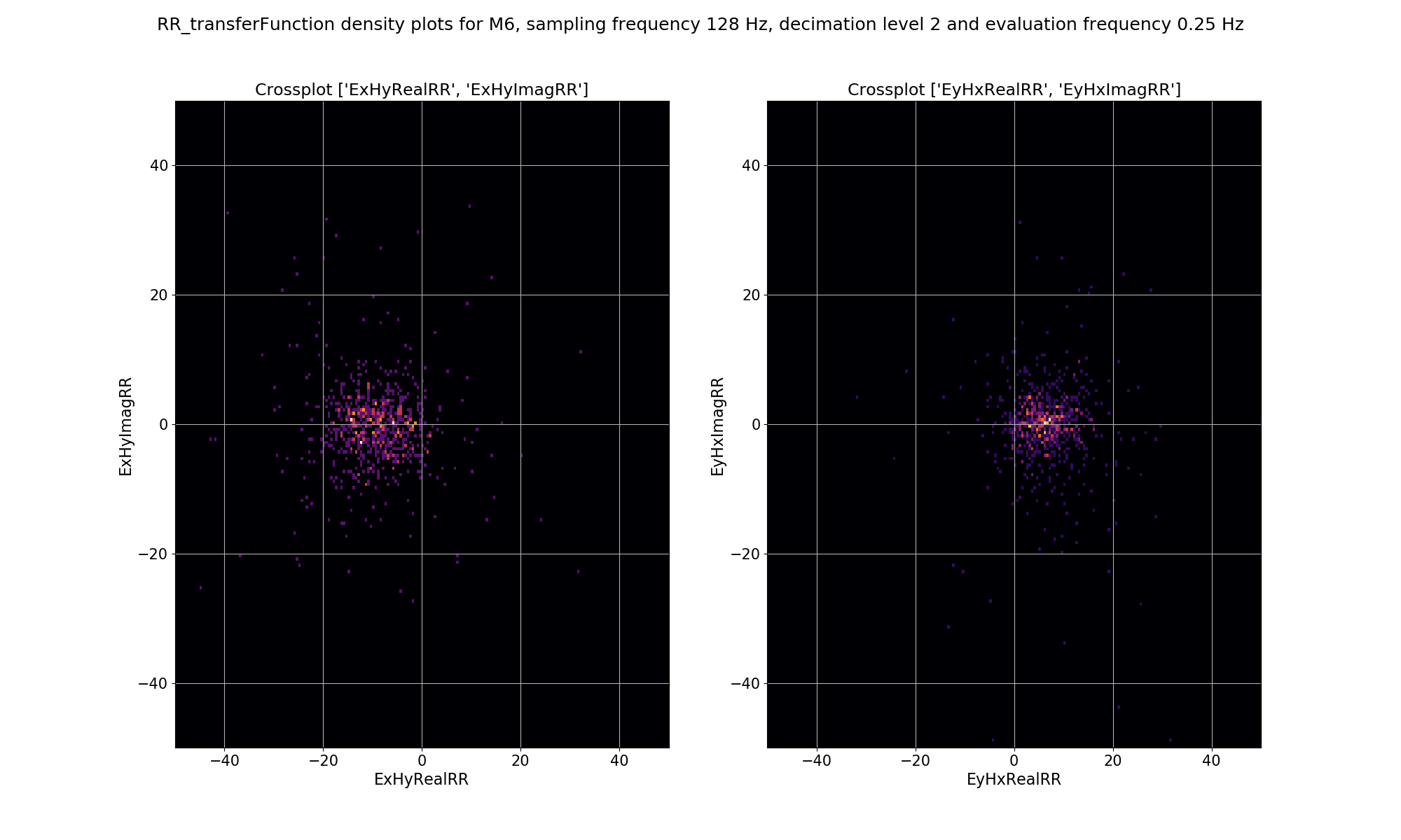
For remote reference statistics, the window-by-window impedance tensor estimates are calculated in the “RR_transferFunction” statistic. This has components: ExHxRealRR, ExHxImagRR, ExHyRealRR, ExHyImagRR, EyHxRealRR, EyHxImagRR, EyHyRealRR, EyHyImagRR. For the density plot, the cross pairs ExHyRealRR vs. ExHyImagRR and EyHxRealRR vs. EyHxImagRR are plotted. This is essentially the Ex-Hy and Ey-Hx polarisations of the remote reference impedance tensor estimates plotted in the complex plane.
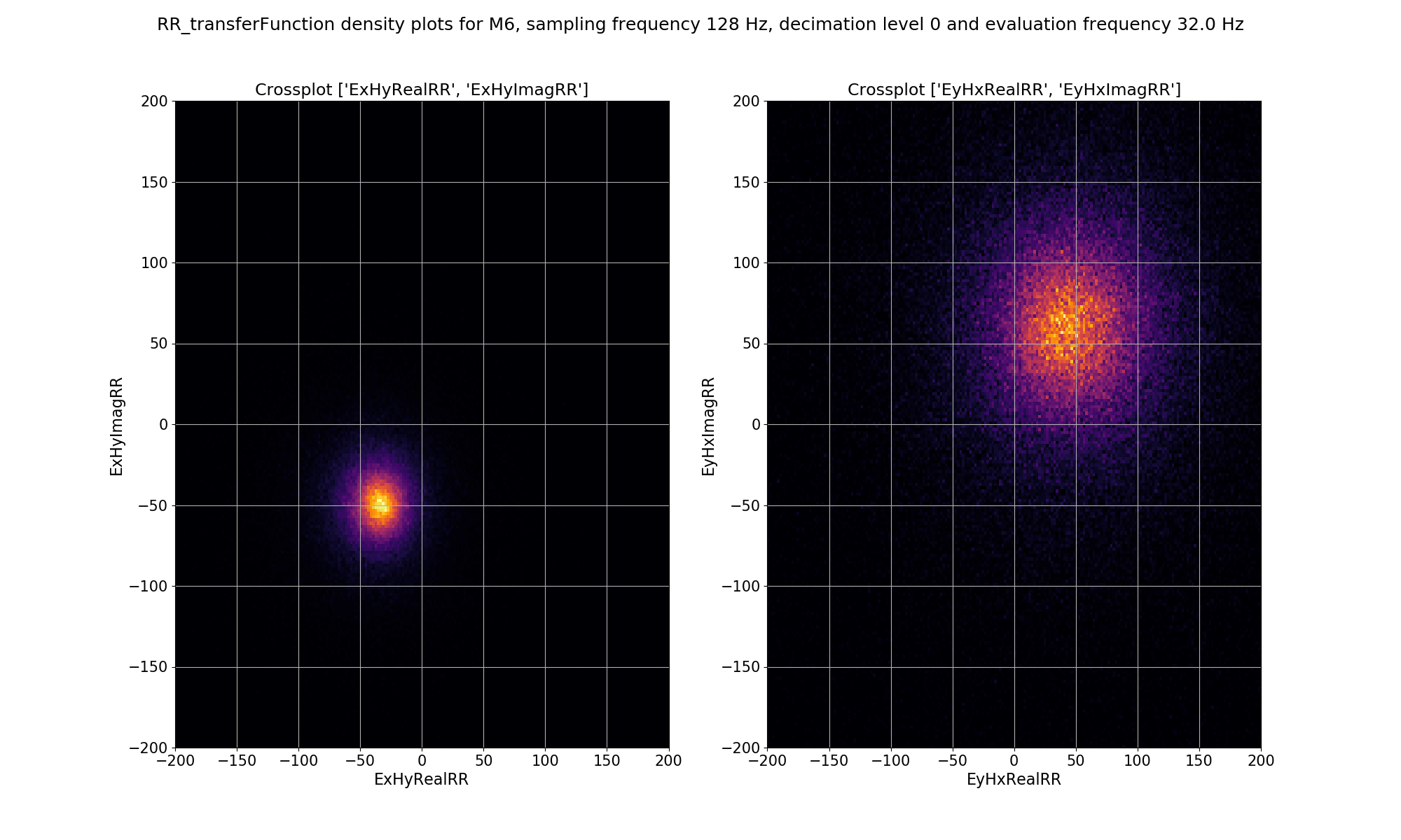
Density plot of remote reference, window-by-window, impedance tensor Ex-Hy and Ey-Hx estimates for decimation level 0, evaluation frequency 32 Hz or period 0.03125 seconds.
The same plots for decimation level 2 are shown below.
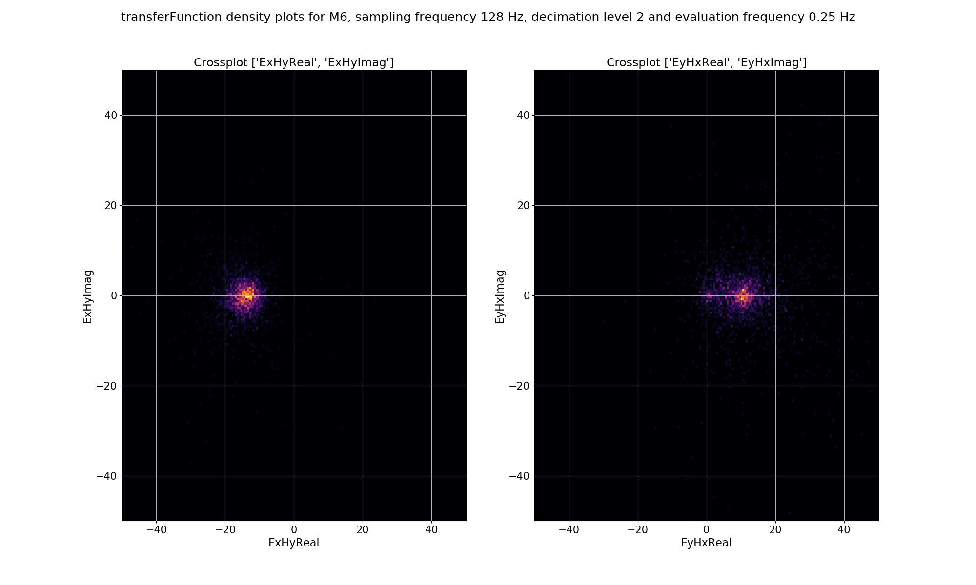
Density plot of single site, window-by-window, impedance tensor Ex-Hy and Ey-Hx estimates for decimation level 2, evaluation frequency 0.25 Hz or period 4 seconds.
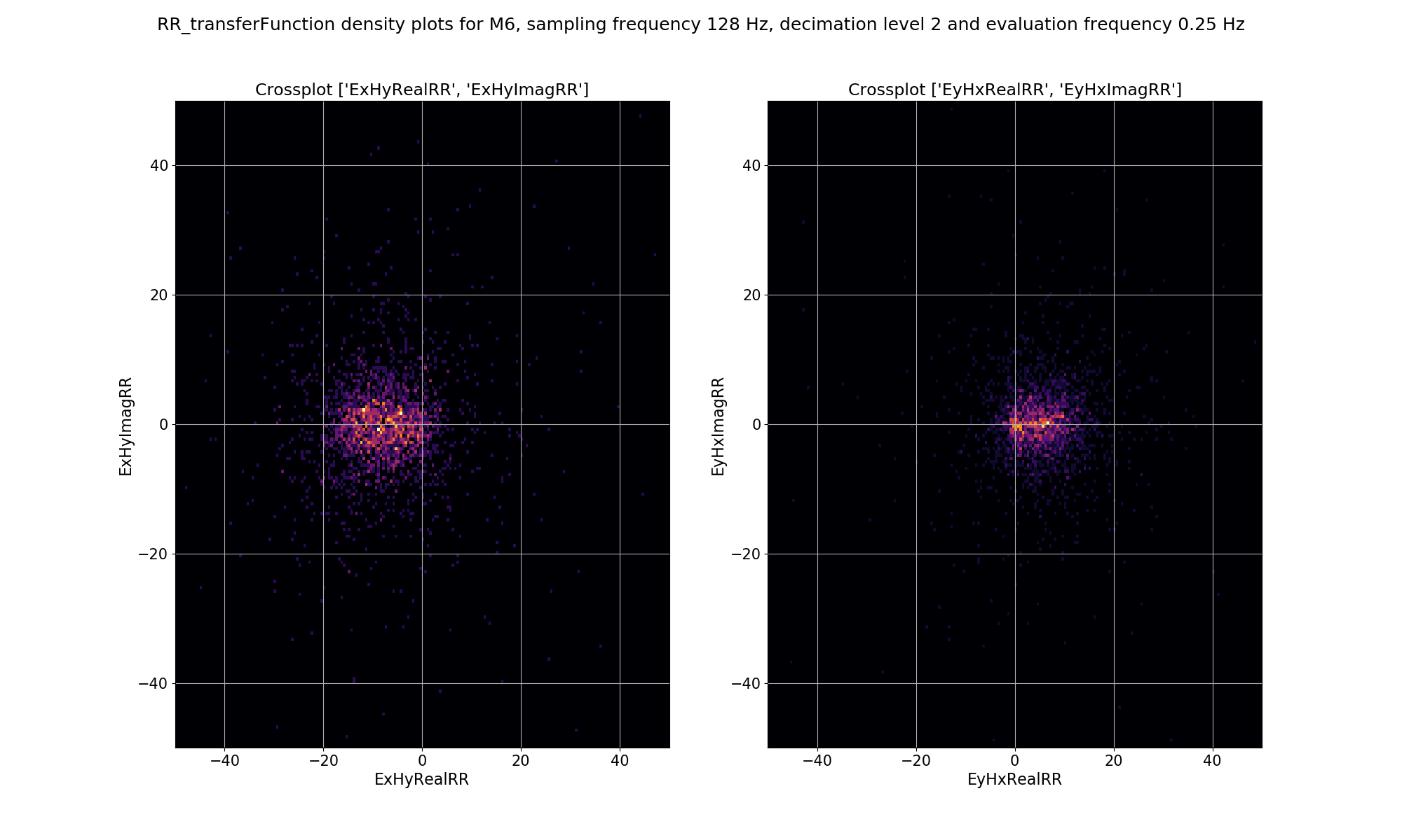
Density plot of remote reference, window-by-window, impedance tensor Ex-Hy and Ey-Hx estimates for decimation level 2, evaluation frequency 0.25 Hz or period 4 seconds.
The plots demonstrate how adding a remote reference is having an impact on the impedance tensor estimates. Particularly the plots for decimation level 2 (period 4 seconds) in the dead band show that by adding the remote reference, not only are the impedance tensor estimates changing, but the spread is becoming larger. Below are the single site impedance tensor estimates for Site M6 and the standard remote reference imepdance tensor estimate for Site M6. Visible in the impedance tensor plots is that the single site phase is smooth (though probably biased) in the dead band, whilst for the same periods, the remote reference estimates show significantly more noise. This is due to the greater spread in window-by-window impedance tensor estimates apparent in the remote reference processing.
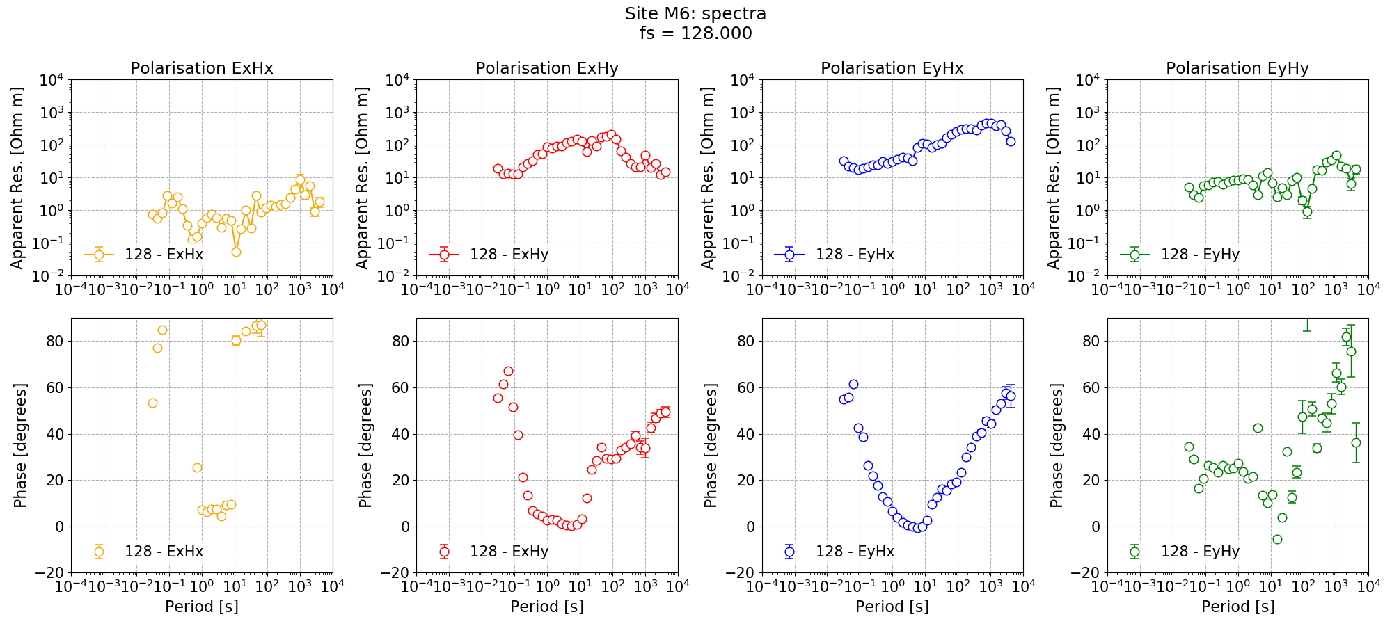
Single site impedance tensor estimates for Site M6 at 128 Hz
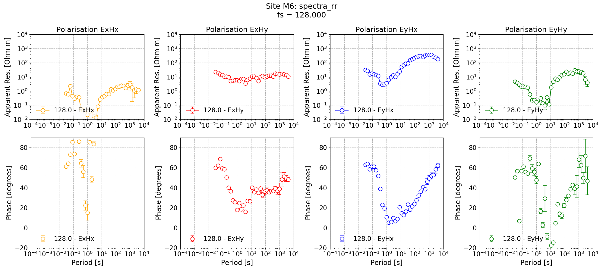
Standard remote reference impedance tensor estimate for Site M6.
Masking with remote reference statistics
Now, the remote reference statistics can be used to generate a mask. The easiest one to use is the remote reference equivalent of coherence. The statistic for this is “RR_coherenceEqn”. Below, a mask is generated for “RR_coherenceEqn” requiring a minimum coherence of 0.8 for the pairs “ExHyR-HyHyR” and “EyHxR-HxHxR”.
59 60 61 62 63 64 65 66 67 68 69 | # create a mask that uses some of the remote reference statistics that were calculated
# get a mask data object and specify the sampling frequency to mask (128Hz)
maskData = newMaskData(proj, 128)
maskData.setStats(["RR_coherenceEqn"])
maskData.addConstraint(
"RR_coherenceEqn", {"ExHyR-HyHyR": [0.8, 1.0], "EyHxR-HxHxR": [0.8, 1.0]}
)
# finally, lets give maskData a name, which will relate to the output file
maskData.maskName = "rr_cohEqn_80_100"
calculateMask(proj, maskData, sites=["M6"])
maskData.printInfo()
|
Important
Because remote reference statistics are always associated with the local site, any masks generated from them are also saved to the local site.
Now, the Site M6 can be remote reference processed using the new mask and the impedance tensor estimate plotted.
71 72 73 74 75 76 77 78 79 80 81 82 83 84 85 86 87 88 89 90 91 92 93 94 | # process with masks
processProject(
proj,
sites=["M6"],
sampleFreqs=[128],
remotesite="Remote",
masks={"M6": "rr_cohEqn_80_100"},
postpend="rr_cohEqn_80_100",
)
from resistics.common.plot import plotOptionsTransferFunction
plotOptionsTF = plotOptionsTransferFunction(plotfonts=getPaperFonts())
figs = viewImpedance(
proj,
sites=["M6"],
sampleFreqs=[128],
postpend="rr_cohEqn_80_100",
oneplot=False,
plotoptions=plotOptionsTF,
save=False,
show=False,
)
figs[0].savefig(remoteImages / "remoteReferenceM6_128_RR_coh.png")
|
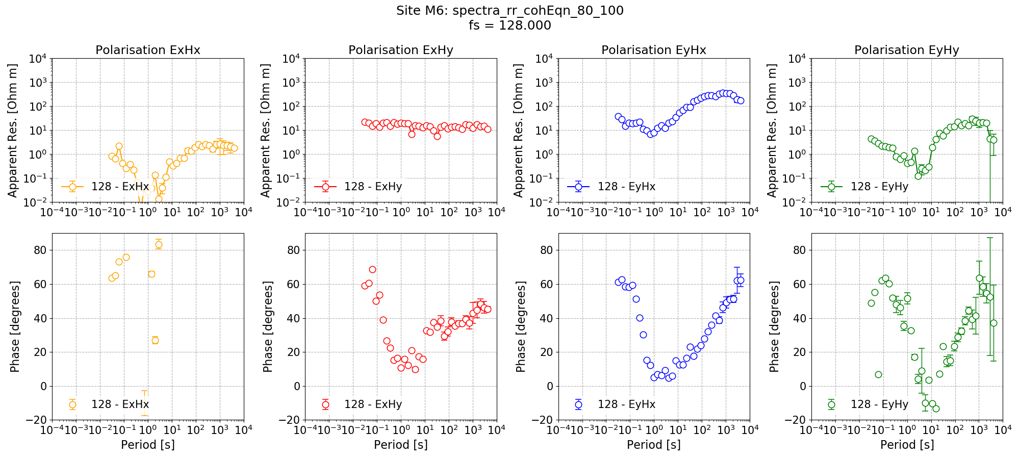
Remote reference impedance tensor estimate for Site M6 using a mask created from remote reference statistics.
It is also possible to see how the mask has affected the density plot by providing a mask into the viewStatisticDensityplot() of module statistics. An example is shown below.
96 97 98 99 100 101 102 103 104 105 106 107 108 109 110 111 112 | # see how the masks changed the density plot
lims = {0: 200, 1: 120, 2: 50, 3: 30}
for declevel in range(0, 4):
fig = viewStatisticDensityplot(
proj,
"M6",
128,
"RR_transferFunction",
declevel=declevel,
crossplots=[["ExHyRealRR", "ExHyImagRR"], ["EyHxRealRR", "EyHxImagRR"]],
maskname="rr_cohEqn_80_100",
xlim=[-lims[declevel], lims[declevel]],
ylim=[-lims[declevel], lims[declevel]],
plotoptions=plotOptions,
show=False,
)
fig.savefig(remoteImages / "densityPlot_remoteRef_{}_mask.png".format(declevel))
|
The effect of masking on the density plot for remote reference impedance tensor estimates for Site M6 and decimation level 2, evaluation frequency 0.25 Hz and period 4 seconds.
Masks and date or time constraints
Recall, however, that masks can be combined with other masks as well as with datetime constraints. In the following example, the remote reference processing is performed again, but with the addition of a datetime constraint which includes only data recorded during the night.
114 115 116 117 118 119 120 121 122 123 124 125 126 127 128 129 130 131 132 133 134 135 | # process with masks and datetime constraints
processProject(
proj,
sites=["M6"],
sampleFreqs=[128],
remotesite="Remote",
masks={"M6": "rr_cohEqn_80_100"},
datetimes=[{"type": "time", "start": "20:00:00", "stop": "07:00:00"}],
postpend="rr_cohEqn_80_100_night",
)
figs = viewImpedance(
proj,
sites=["M6"],
sampleFreqs=[128],
postpend="rr_cohEqn_80_100_night",
oneplot=False,
plotoptions=plotOptionsTF,
save=False,
show=False,
)
figs[0].savefig(remoteImages / "remoteReferenceM6_128_RR_coh_datetime.png")
|
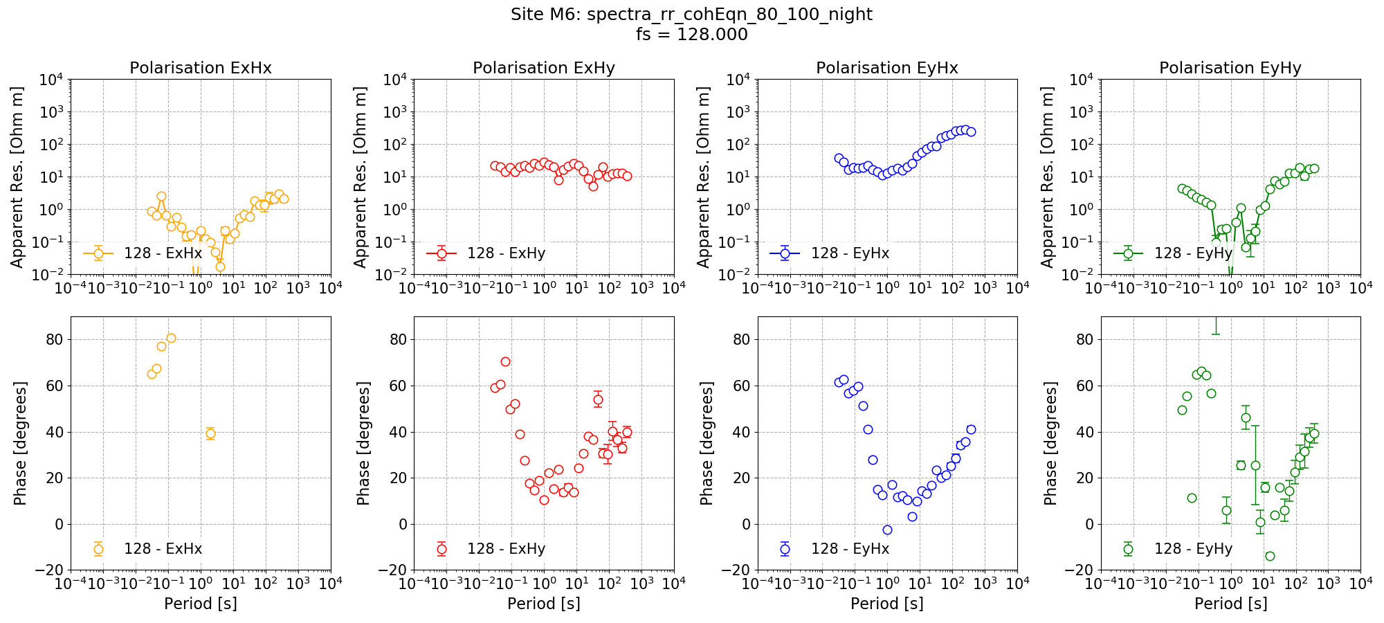
Remote reference impedance tensor estimate for Site M6 using a mask created from remote reference statistics and with additional time constraints.
The new impedance tensor esimate appears better at the low decimation levels where there are plently of windows and worse at the high decimation levels where it is reducing the number of windows which can be included in the processing. The remote reference processing can be performed again, but this time applying the time constraints only to decimation levels 0 and 1.
137 138 139 140 141 142 143 144 145 146 147 148 149 150 151 152 153 154 155 156 157 158 159 160 | # process with masks and datetime constraints, but only for decimation levels 0 and 1
processProject(
proj,
sites=["M6"],
sampleFreqs=[128],
remotesite="Remote",
masks={"M6": "rr_cohEqn_80_100"},
datetimes=[
{"type": "time", "start": "20:00:00", "stop": "07:00:00", "levels": [0, 1]}
],
postpend="rr_cohEqn_80_100_night2",
)
figs = viewImpedance(
proj,
sites=["M6"],
sampleFreqs=[128],
postpend="rr_cohEqn_80_100_night2",
oneplot=False,
plotoptions=plotOptionsTF,
save=False,
show=False,
)
figs[0].savefig(remoteImages / "remoteReferenceM6_128_RR_coh_datetime_01.png")
|
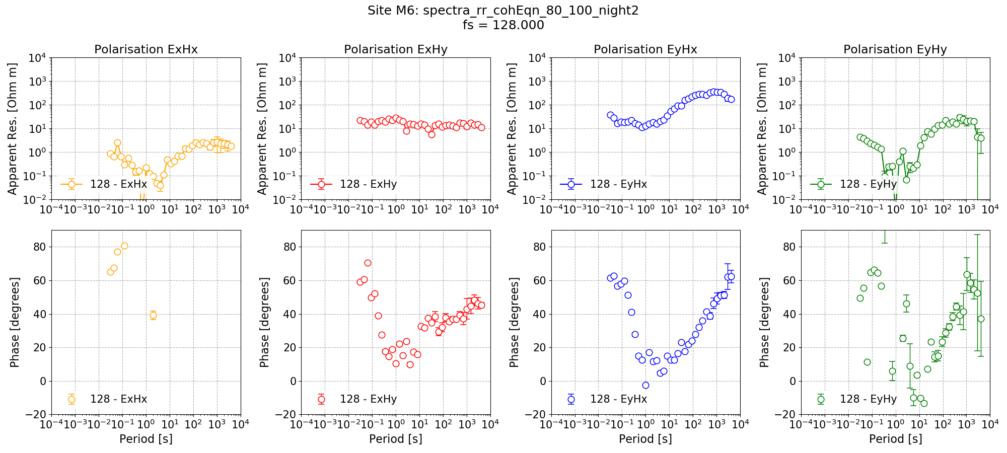
Remote reference impedance tensor estimate for Site M6 using a mask created from remote reference statistics and with additional time constraints only applied to decimation levels 0 and 1.
Complete example script
For the purposes of clarity, the complete example script is provided below.
1 2 3 4 5 6 7 8 9 10 11 12 13 14 15 16 17 18 19 20 21 22 23 24 25 26 27 28 29 30 31 32 33 34 35 36 37 38 39 40 41 42 43 44 45 46 47 48 49 50 51 52 53 54 55 56 57 58 59 60 61 62 63 64 65 66 67 68 69 70 71 72 73 74 75 76 77 78 79 80 81 82 83 84 85 86 87 88 89 90 91 92 93 94 95 96 97 98 99 100 101 102 103 104 105 106 107 108 109 110 111 112 113 114 115 116 117 118 119 120 121 122 123 124 125 126 127 128 129 130 131 132 133 134 135 136 137 138 139 140 141 142 143 144 145 146 147 148 149 150 151 152 153 154 155 156 157 158 159 160 | from datapaths import remotePath, remoteImages
from resistics.project.io import loadProject
from resistics.project.statistics import (
calculateRemoteStatistics,
viewStatistic,
viewStatisticHistogram,
viewStatisticDensityplot,
)
from resistics.project.mask import newMaskData, calculateMask
from resistics.project.transfunc import processProject, viewImpedance
from resistics.common.plot import plotOptionsStandard, getPaperFonts
plotOptions = plotOptionsStandard(plotfonts=getPaperFonts())
proj = loadProject(remotePath)
calculateRemoteStatistics(
proj,
"Remote",
sites=["M6"],
sampleFreqs=[128],
remotestats=[
"RR_coherence",
"RR_coherenceEqn",
"RR_absvalEqn",
"RR_transferFunction",
"RR_resPhase",
],
)
lims = {0: 200, 1: 120, 2: 50, 3: 30}
for declevel in range(0, 4):
    fig = viewStatisticDensityplot(
        proj,
        "M6",
        128,
        "RR_transferFunction",
        declevel=declevel,
        crossplots=[["ExHyRealRR", "ExHyImagRR"], ["EyHxRealRR", "EyHxImagRR"]],
        xlim=[-lims[declevel], lims[declevel]],
        ylim=[-lims[declevel], lims[declevel]],
        plotoptions=plotOptions,
        show=False,
    )
    fig.savefig(remoteImages / "densityPlot_remoteRef_{}.png".format(declevel))
    fig = viewStatisticDensityplot(
        proj,
        "M6",
        128,
        "transferFunction",
        declevel=declevel,
        crossplots=[["ExHyReal", "ExHyImag"], ["EyHxReal", "EyHxImag"]],
        xlim=[-lims[declevel], lims[declevel]],
        ylim=[-lims[declevel], lims[declevel]],
        plotoptions=plotOptions,
        show=False,
    )
    fig.savefig(remoteImages / "densityPlot_singleSite_{}.png".format(declevel))
# create a mask that uses some of the remote reference statistics that were calculated
# get a mask data object and specify the sampling frequency to mask (128Hz)
maskData = newMaskData(proj, 128)
maskData.setStats(["RR_coherenceEqn"])
maskData.addConstraint(
    "RR_coherenceEqn", {"ExHyR-HyHyR": [0.8, 1.0], "EyHxR-HxHxR": [0.8, 1.0]}
)
# finally, lets give maskData a name, which will relate to the output file
maskData.maskName = "rr_cohEqn_80_100"
calculateMask(proj, maskData, sites=["M6"])
maskData.printInfo()
# process with masks
processProject(
    proj,
    sites=["M6"],
    sampleFreqs=[128],
    remotesite="Remote",
    masks={"M6": "rr_cohEqn_80_100"},
    postpend="rr_cohEqn_80_100",
)

from resistics.common.plot import plotOptionsTransferFunction

plotOptionsTF = plotOptionsTransferFunction(plotfonts=getPaperFonts())
figs = viewImpedance(
    proj,
    sites=["M6"],
    sampleFreqs=[128],
    postpend="rr_cohEqn_80_100",
    oneplot=False,
    plotoptions=plotOptionsTF,
    save=False,
    show=False,
)
figs[0].savefig(remoteImages / "remoteReferenceM6_128_RR_coh.png")
# see how the masks changed the density plot
lims = {0: 200, 1: 120, 2: 50, 3: 30}
for declevel in range(0, 4):
    fig = viewStatisticDensityplot(
        proj,
        "M6",
        128,
        "RR_transferFunction",
        declevel=declevel,
        crossplots=[["ExHyRealRR", "ExHyImagRR"], ["EyHxRealRR", "EyHxImagRR"]],
        maskname="rr_cohEqn_80_100",
        xlim=[-lims[declevel], lims[declevel]],
        ylim=[-lims[declevel], lims[declevel]],
        plotoptions=plotOptions,
        show=False,
    )
    fig.savefig(remoteImages / "densityPlot_remoteRef_{}_mask.png".format(declevel))
# process with masks and datetime constraints
processProject(
    proj,
    sites=["M6"],
    sampleFreqs=[128],
    remotesite="Remote",
    masks={"M6": "rr_cohEqn_80_100"},
    datetimes=[{"type": "time", "start": "20:00:00", "stop": "07:00:00"}],
    postpend="rr_cohEqn_80_100_night",
)

figs = viewImpedance(
    proj,
    sites=["M6"],
    sampleFreqs=[128],
    postpend="rr_cohEqn_80_100_night",
    oneplot=False,
    plotoptions=plotOptionsTF,
    save=False,
    show=False,
)
figs[0].savefig(remoteImages / "remoteReferenceM6_128_RR_coh_datetime.png")
# process with masks and datetime constraints, but only for decimation levels 0 and 1
processProject(
    proj,
    sites=["M6"],
    sampleFreqs=[128],
    remotesite="Remote",
    masks={"M6": "rr_cohEqn_80_100"},
    datetimes=[
        {"type": "time", "start": "20:00:00", "stop": "07:00:00", "levels": [0, 1]}
    ],
    postpend="rr_cohEqn_80_100_night2",
)

figs = viewImpedance(
    proj,
    sites=["M6"],
    sampleFreqs=[128],
    postpend="rr_cohEqn_80_100_night2",
    oneplot=False,
    plotoptions=plotOptionsTF,
    save=False,
    show=False,
)
figs[0].savefig(remoteImages / "remoteReferenceM6_128_RR_coh_datetime_01.png")
|