Intersite transfer functions
Intesite transfer functions use input channels from one site and output channels from another. In magnetotellurics, the input sites are usually magnetic and the output electric. In field surveys intended for intersite transfer functions, there are often many sites that record electric channels only.
In the following example, the data used will be:
Data from a Lemi B423 MT station. This data is used in the Processing Lemi B423 data example.
Data from a Lemi B423 telluric station recording only electric channels.
And from the perspective of the magnetotelluric transfer function:
The telluric site is the output site as the electric channels are the output of the standard magnetotelluric impedance tensor formulation.
The magnetotelluric site is the input site as the magnetic channels are the input of the standard magnetotelluric impedance tensor formulation.
Note
It is recommend to read the Processing Lemi B423 data example in the cookbook before following this tutorial to understand more about Lemi B423 data.
The steps that will be followed are:
Create the project and organise the data (magnetotelluric, telluric and calibration)
Create the Lemi B423 headers and B423E headers
Define the configuration to use (based on the results in Processing Lemi B423 data)
Calculate spectra (and statistics for the MT site)
Process to estimate the intersite impedance tensor
Begin by creating the project,
1 2 3 4 5 | from datapaths import intersitePath
from resistics.project.io import newProject
refTime = "2019-05-27 00:00:00"
newProject(intersitePath, refTime)
|
Copy the data in there to give this structure:
usingLemi
├── calData
│   ├── lemi120_IC_710.txt
│   ├── lemi120_IC_712.txt
│   └── lemi120_IC_714.txt
├── timeData
│   ├── site1_mt
│   │   └── lemi01
│   │       ├── 1558950203.B423
│   │       ├── 1558961007.B423
│   │       ├── 1558971807.B423
│   │       ├── 1558982607.B423
│   │       ├── 1558993407.B423
│   │       ├── 1559004207.B423
│   │       ├── 1559015007.B423
│   │       └── 1559025807.B423
│   └── site2_te
│       └── lemi01
│           ├── 1558948829.B423
│           ├── 1558959633.B423
│           ├── 1558970433.B423
│           ├── 1558981233.B423
│           ├── 1558992033.B423
│           ├── 1559002833.B423
│           ├── 1559013633.B423
│           ├── 1559024433.B423
│           ├── 1559035233.B423
│           ├── 1559046033.B423
│           ├── 1559056833.B423
│           ├── 1559067633.B423
│           ├── 1559078433.B423
│           └── 1559089233.B423
├── specData
├── statData
├── maskData
├── transFuncData
├── images
└── mtProj.prj
The next stage is to create the headers for both the magnetotelluric and telluric data.
1 2 3 4 5 6 7 8 9 10 11 12 13 14 15 16 17 18 19 20 21 22 23 | from datapaths import intersitePath, intersiteImages
from resistics.project.io import loadProject
# headers for MT stations
from resistics.time.reader_lemib423 import folderB423Headers
folderB423Headers(
intersitePath / "timeData" / "site1_mt",
500,
hxSensor=712,
hySensor=710,
hzSensor=714,
hGain=16,
dx=60,
dy=60.7,
)
# headers for telluric only stations
from resistics.time.reader_lemib423e import folderB423EHeaders
folderB423EHeaders(
intersitePath / "timeData" / "site2_te", 500, ex="E1", ey="E2", dx=60, dy=60.7
)
|
After running this section, the project now looks like:
usingLemi
├── calData
│   ├── lemi120_IC_710.txt
│   ├── lemi120_IC_712.txt
│   └── lemi120_IC_714.txt
├── timeData
│   ├── site1_mt
│   │   └── lemi01
│   │       ├── 1558950203.B423
│   │       ├── 1558961007.B423
│   │       ├── 1558971807.B423
│   │       ├── 1558982607.B423
│   │       ├── 1558993407.B423
│   │       ├── 1559004207.B423
│   │       ├── 1559015007.B423
│   │       ├── 1559025807.B423
│   │       ├── chan_00.h423
│   │       ├── chan_01.h423
│   │       ├── chan_02.h423
│   │       ├── chan_03.h423
│   │       ├── chan_04.h423
│   │       └── global.h423
│   └── site2_te
│       └── lemi01
│           ├── 1558948829.B423
│           ├── 1558959633.B423
│           ├── 1558970433.B423
│           ├── 1558981233.B423
│           ├── 1558992033.B423
│           ├── 1559002833.B423
│           ├── 1559013633.B423
│           ├── 1559024433.B423
│           ├── 1559035233.B423
│           ├── 1559046033.B423
│           ├── 1559056833.B423
│           ├── 1559067633.B423
│           ├── 1559078433.B423
│           ├── 1559089233.B423
│           ├── chan_00.h423
│           ├── chan_01.h423
│           ├── chan_02.h423
│           ├── chan_03.h423
│           └── global.h423
├── specData
├── statData
├── maskData
├── transFuncData
├── images
└── mtProj.prj
The headers for the magnetotellruic and telluric data have been generated and the project can be loaded and the project timeline plotted.
29 30 31 32 33 | # load the project
proj = loadProject(intersitePath, "customconfig.ini")
proj.printInfo()
fig = proj.view()
fig.savefig(intersiteImages / "timeline.png")
|
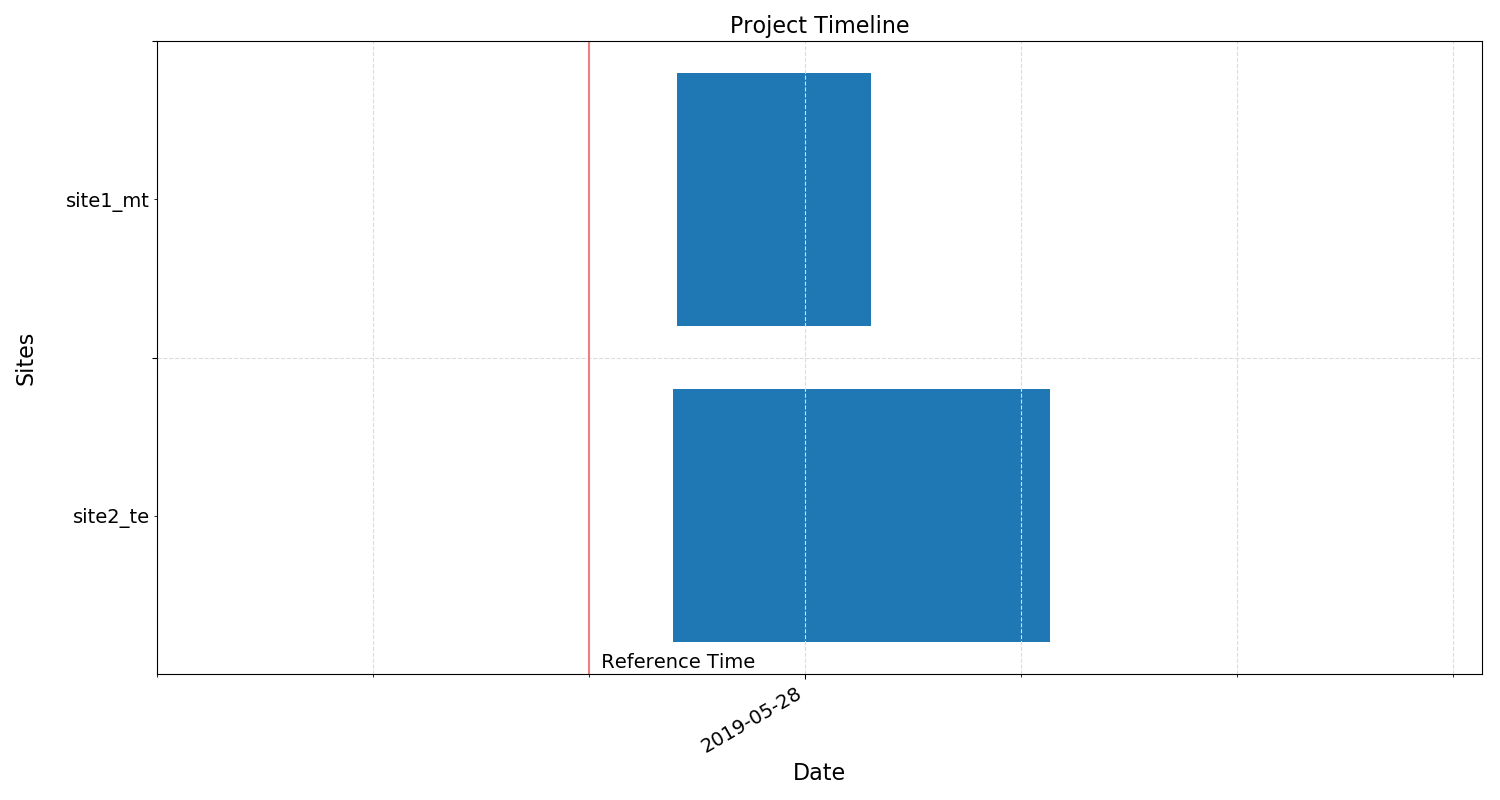
Project timeline
The configuration that will be used is the same that was used in the Processing Lemi B423 data example, which has more information about why that configuration was chosen. The configuration parameters are shown below.
1 2 3 4 5 6 7 8 9 10 11 | name = customwin
[Spectra]
specdir = "customwin"
[Window]
windowsizes = 1024, 512, 256, 256, 128, 128, 128
overlapsizes = 256, 128, 64, 64, 32, 32, 32
[Statistics]
stats = "coherence", "transferFunction",
|
Time data can be viewed in the usual way with the viewTime() method.
31 32 33 34 35 36 37 38 39 40 41 42 | # view time
from resistics.project.time import viewTime
fig = viewTime(
proj,
startDate="2019-05-27 14:15:00",
endDate="2019-05-27 15:00:00",
filter={"lpfilt": 4},
save=False,
show=False,
)
fig.savefig(intersiteImages / "viewTime.png")
|
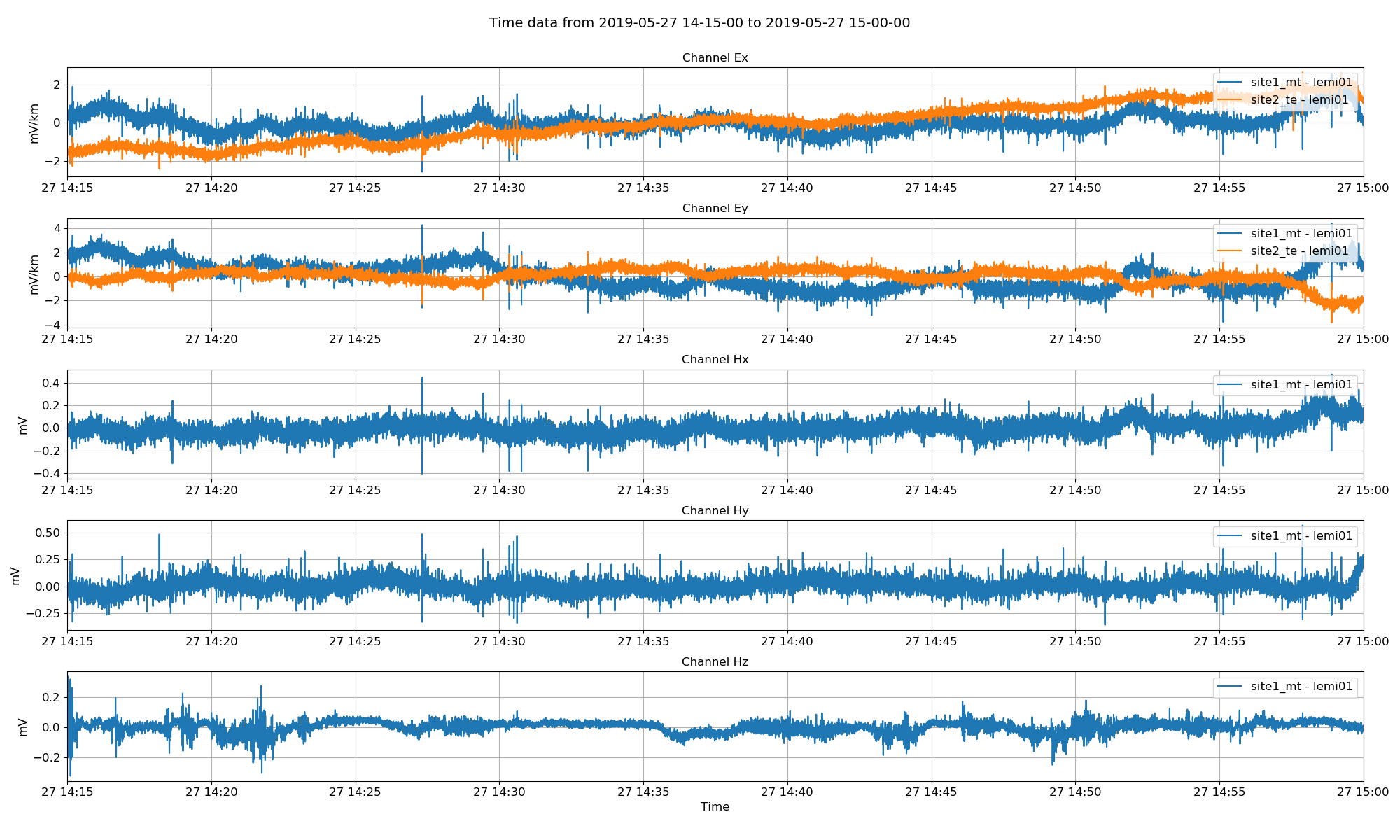
Viewing time series data. It appears as though the Ey for the telluric data needs to be reversed.
From looking at the time series plot, the Ey channel of the telluric station needs a polarity reversal (multiply by -1). This can be done when calculating out spectra as shown below.
44 45 46 47 48 49 50 51 | # calculate spectra
from resistics.project.spectra import calculateSpectra
calculateSpectra(proj, sites=["site1_mt"])
calculateSpectra(
proj, sites=["site2_te"], chans=["Ex", "Ey"], polreverse={"Ey": True}
)
proj.refresh()
|
Now, statistics can be calculated for the magnetotelluric site.
Note
There are no useful statistics at this moment for telluric sites nor are there intersite statistics.
53 54 55 56 | # calculate statistics for MT site
from resistics.project.statistics import calculateStatistics
calculateStatistics(proj, sites=["site1_mt"])
|
With the statistics calculated, the intersite processing can be performed, initially without any statistic based masking.
58 59 60 61 62 63 64 65 66 67 68 69 70 71 72 73 74 75 76 77 78 79 80 81 82 83 84 | # intersite
from resistics.project.transfunc import (
processProject,
processSite,
viewImpedance,
)
from resistics.common.plot import plotOptionsTransferFunction, getPaperFonts
plotOptions = plotOptionsTransferFunction(figsize=(24, 12), plotfonts=getPaperFonts())
plotOptions["res_ylim"] = [1, 1000000]
processSite(
proj,
"site2_te",
500,
inputsite="site1_mt",
postpend="intersite",
)
figs = viewImpedance(
proj,
sites=["site2_te"],
postpend="intersite",
plotoptions=plotOptions,
oneplot=False,
save=False,
show=False,
)
figs[0].savefig(intersiteImages / "intersiteTransferFunction.png")
|
The important call in this section of code is the call to processSite(). In this call, we have set the output site as “site2_te” or the telluric site. The optional input of inputsite has been set to the magnetotellruic site, site1_mt. The result of this is:
electric channel data will be taken from site2_te or the telluric site
magnetic channel data will be take from site1_mt or the magnetotelluric site
The resultant intersite transfer function is shown below.
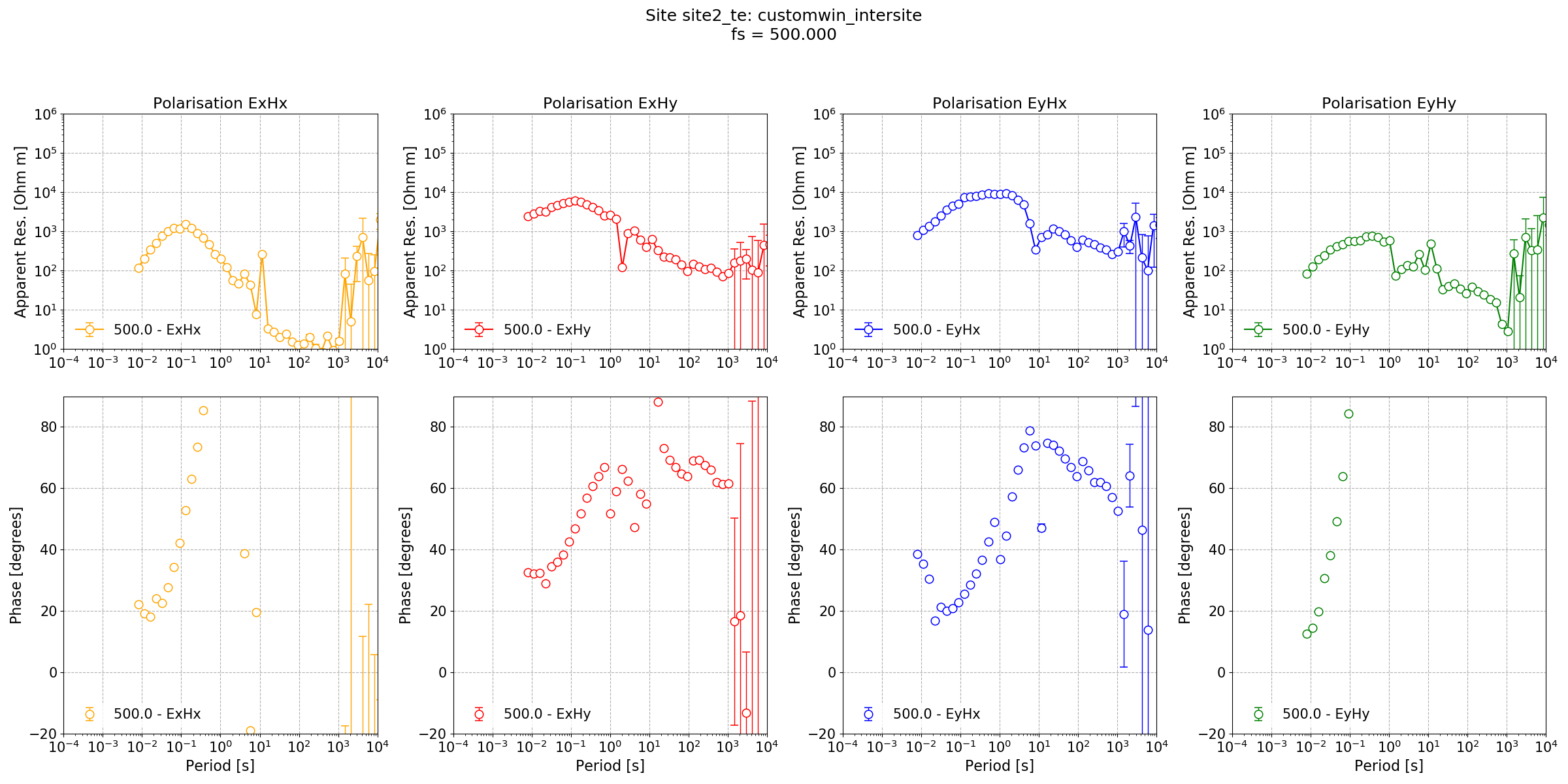
Intersite transfer function.
In the Processing Lemi B423 data example, a significantly better result was achieved using a varying coherence mask. The same can be done here, but the mask will only be based on the quality of the data at the magnetotelluric site as no statistics were calculated for the telluric site.
86 87 88 89 90 91 92 93 94 95 96 97 98 99 100 101 102 103 104 105 106 107 108 109 110 111 112 113 114 115 116 117 118 119 120 121 122 123 124 125 126 127 128 129 130 131 132 133 | # now try again with some statistics for the dead band
from resistics.project.mask import newMaskData, calculateMask
maskData = newMaskData(proj, 500)
maskData.setStats(["coherence"])
maskData.addConstraintLevel(
"coherence", {"cohExHy": [0.8, 1.0], "cohEyHx": [0.8, 1.0]}, 0
)
maskData.addConstraintLevel(
"coherence", {"cohExHy": [0.8, 1.0], "cohEyHx": [0.8, 1.0]}, 1
)
maskData.addConstraintLevel(
"coherence", {"cohExHy": [0.7, 1.0], "cohEyHx": [0.7, 1.0]}, 2
)
maskData.addConstraintLevel(
"coherence", {"cohExHy": [0.6, 1.0], "cohEyHx": [0.6, 1.0]}, 3
)
maskData.addConstraintLevel(
"coherence", {"cohExHy": [0.5, 1.0], "cohEyHx": [0.5, 1.0]}, 4
)
maskData.addConstraintLevel(
"coherence", {"cohExHy": [0.5, 1.0], "cohEyHx": [0.5, 1.0]}, 5
)
maskData.addConstraintLevel(
"coherence", {"cohExHy": [0.4, 1.0], "cohEyHx": [0.4, 1.0]}, 6
)
maskData.maskName = "coh80_100"
calculateMask(proj, maskData, sites=["site1_mt"])
# process with mask
processSite(
proj,
"site2_te",
500,
inputsite="site1_mt",
masks={"site1_mt": "coh80_100"},
postpend="intersite_coh80_100",
)
figs = viewImpedance(
proj,
sites=["site2_te"],
postpend="intersite_coh80_100",
plotoptions=plotOptions,
oneplot=False,
save=False,
show=False,
)
figs[0].savefig(intersiteImages / "intersiteTransferFunctionMask.png")
|
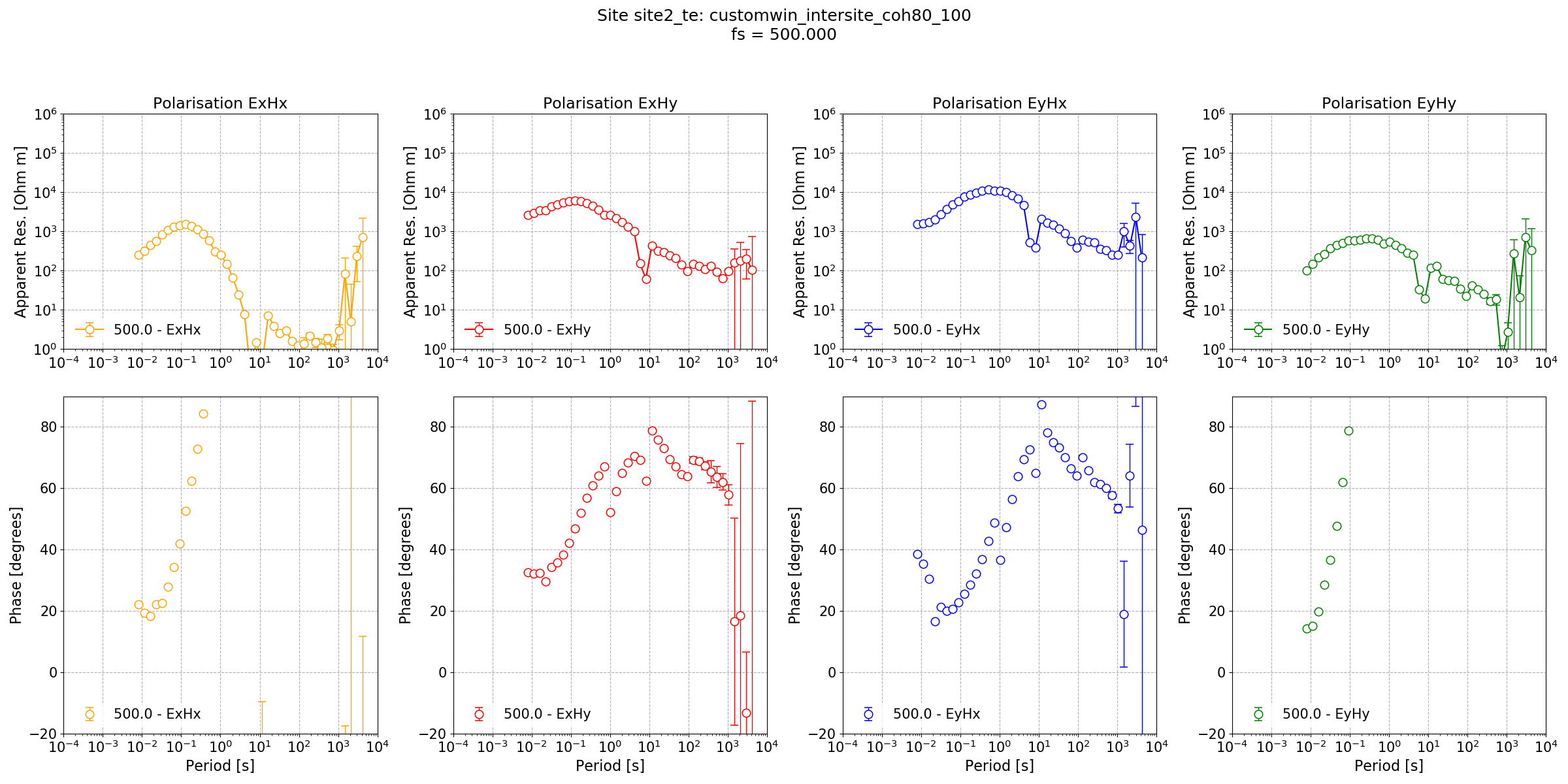
The intersite transfer function with variable masking
There is still problems with the output at long periods, most noticeably in the phase. This is likely to be a synchronisation issue between the two sites.
Complete example scripts
For the purposes of clarity, the complete example scripts is provided below.
Creating the project.
1 2 3 4 5 | from datapaths import intersitePath
from resistics.project.io import newProject
refTime = "2019-05-27 00:00:00"
newProject(intersitePath, refTime)
|
Processing intersite transfer function.
1 2 3 4 5 6 7 8 9 10 11 12 13 14 15 16 17 18 19 20 21 22 23 24 25 26 27 28 29 30 31 32 33 34 35 36 37 38 39 40 41 42 43 44 45 46 47 48 49 50 51 52 53 54 55 56 57 58 59 60 61 62 63 64 65 66 67 68 69 70 71 72 73 74 75 76 77 78 79 80 81 82 83 84 85 86 87 88 89 90 91 92 93 94 95 96 97 98 99 100 101 102 103 104 105 106 107 108 109 110 111 112 113 114 115 116 117 118 119 120 121 122 123 124 125 126 127 128 129 130 131 132 133 | from datapaths import intersitePath, intersiteImages
from resistics.project.io import loadProject
# headers for MT stations
from resistics.time.reader_lemib423 import folderB423Headers
folderB423Headers(
intersitePath / "timeData" / "site1_mt",
500,
hxSensor=712,
hySensor=710,
hzSensor=714,
hGain=16,
dx=60,
dy=60.7,
)
# headers for telluric only stations
from resistics.time.reader_lemib423e import folderB423EHeaders
folderB423EHeaders(
intersitePath / "timeData" / "site2_te", 500, ex="E1", ey="E2", dx=60, dy=60.7
)
# load the project
proj = loadProject(intersitePath, "customconfig.ini")
proj.printInfo()
fig = proj.view()
fig.savefig(intersiteImages / "timeline.png")
# view time
from resistics.project.time import viewTime

fig = viewTime(
    proj,
    startDate="2019-05-27 14:15:00",
    endDate="2019-05-27 15:00:00",
    filter={"lpfilt": 4},
    save=False,
    show=False,
)
fig.savefig(intersiteImages / "viewTime.png")
# calculate spectra
from resistics.project.spectra import calculateSpectra

calculateSpectra(proj, sites=["site1_mt"])
calculateSpectra(
    proj, sites=["site2_te"], chans=["Ex", "Ey"], polreverse={"Ey": True}
)
proj.refresh()
# calculate statistics for MT site
from resistics.project.statistics import calculateStatistics

calculateStatistics(proj, sites=["site1_mt"])
# intersite
from resistics.project.transfunc import (
    processProject,
    processSite,
    viewImpedance,
)
from resistics.common.plot import plotOptionsTransferFunction, getPaperFonts

plotOptions = plotOptionsTransferFunction(figsize=(24, 12), plotfonts=getPaperFonts())
plotOptions["res_ylim"] = [1, 1000000]
processSite(
    proj,
    "site2_te",
    500,
    inputsite="site1_mt",
    postpend="intersite",
)
figs = viewImpedance(
    proj,
    sites=["site2_te"],
    postpend="intersite",
    plotoptions=plotOptions,
    oneplot=False,
    save=False,
    show=False,
)
figs[0].savefig(intersiteImages / "intersiteTransferFunction.png")
# now try again with some statistics for the dead band
from resistics.project.mask import newMaskData, calculateMask

maskData = newMaskData(proj, 500)
maskData.setStats(["coherence"])
maskData.addConstraintLevel(
    "coherence", {"cohExHy": [0.8, 1.0], "cohEyHx": [0.8, 1.0]}, 0
)
maskData.addConstraintLevel(
    "coherence", {"cohExHy": [0.8, 1.0], "cohEyHx": [0.8, 1.0]}, 1
)
maskData.addConstraintLevel(
    "coherence", {"cohExHy": [0.7, 1.0], "cohEyHx": [0.7, 1.0]}, 2
)
maskData.addConstraintLevel(
    "coherence", {"cohExHy": [0.6, 1.0], "cohEyHx": [0.6, 1.0]}, 3
)
maskData.addConstraintLevel(
    "coherence", {"cohExHy": [0.5, 1.0], "cohEyHx": [0.5, 1.0]}, 4
)
maskData.addConstraintLevel(
    "coherence", {"cohExHy": [0.5, 1.0], "cohEyHx": [0.5, 1.0]}, 5
)
maskData.addConstraintLevel(
    "coherence", {"cohExHy": [0.4, 1.0], "cohEyHx": [0.4, 1.0]}, 6
)
maskData.maskName = "coh80_100"
calculateMask(proj, maskData, sites=["site1_mt"])

# process with mask
processSite(
    proj,
    "site2_te",
    500,
    inputsite="site1_mt",
    masks={"site1_mt": "coh80_100"},
    postpend="intersite_coh80_100",
)
figs = viewImpedance(
    proj,
    sites=["site2_te"],
    postpend="intersite_coh80_100",
    plotoptions=plotOptions,
    oneplot=False,
    save=False,
    show=False,
)
figs[0].savefig(intersiteImages / "intersiteTransferFunctionMask.png")
|