Processing Lemi B423 data
For an introduction to using Lemi B423 data, please see Lemi B423 timeseries.
Like always, begin by setting up a project.
1 2 3 4 5 6 | from datapaths import projectPath
from resistics.project.io import newProject
referenceTime = "2019-05-25 12:00:00"
proj = newProject(projectPath, referenceTime)
proj.printInfo()
|
There is no data in the project currently. To be able to use the Lemi B423 data, it needs to be placed into the project and the appropriate headers made.
The Lemi B423 data is placed as follows:
usingLemi
├── calData
├── timeData
│   └── site1_mt
│       └── lemi01
│           ├── 1558950203.B423
│           ├── 1558961007.B423
│           ├── 1558971807.B423
│           ├── 1558982607.B423
│           ├── 1558993407.B423
│           ├── 1559004207.B423
│           ├── 1559015007.B423
│           └── 1559025807.B423
├── specData
├── statData
├── maskData
├── transFuncData
├── images
└── mtProj.prj
To make the header files, the folderB423Headers() method of module :meth:`~resistics.time.reader_lemib423 is used.
1 2 3 4 5 6 7 8 | from datapaths import projectPath, imagePath
from resistics.time.reader_lemib423 import folderB423Headers
# first need to create headers
sitePath = projectPath / "timeData" / "site1_mt"
folderB423Headers(
sitePath, 500, hxSensor=712, hySensor=710, hzSensor=714, hGain=16, dx=60, dy=60.7
)
|
The project now looks like this:
usingLemi
├── calData
├── timeData
│   └── site1_mt
│       └── lemi01
│           ├── 1558950203.B423
│           ├── 1558961007.B423
│           ├── 1558971807.B423
│           ├── 1558982607.B423
│           ├── 1558993407.B423
│           ├── 1559004207.B423
│           ├── 1559015007.B423
│           ├── 1559025807.B423
│           ├── chan_00.h423
│           ├── chan_01.h423
│           ├── chan_02.h423
│           ├── chan_03.h423
│           ├── chan_04.h423
│           └── global.h423
├── specData
├── statData
├── maskData
├── transFuncData
├── images
└── mtProj.prj
Additionally, calibration files need to be present. These are placed in the calData folder. In this case, ascii calibration files are being used. More about calibration files can be found in Calibration and in particular, about ascii calibration files here.
usingLemi
├── calData
│   ├── lemi120_IC_710.txt
│   ├── lemi120_IC_712.txt
│   └── lemi120_IC_714.txt
├── timeData
│   └── site1_mt
│       └── lemi01
│           ├── 1558950203.B423
│           ├── 1558961007.B423
│           ├── 1558971807.B423
│           ├── 1558982607.B423
│           ├── 1558993407.B423
│           ├── 1559004207.B423
│           ├── 1559015007.B423
│           ├── 1559025807.B423
│           ├── chan_00.h423
│           ├── chan_01.h423
│           ├── chan_02.h423
│           ├── chan_03.h423
│           ├── chan_04.h423
│           └── global.h423
├── specData
├── statData
├── maskData
├── transFuncData
├── images
└── mtProj.prj
Note
For ascii format calibration files, the important thing is that the name is of the format:
[]_IC_[serial number].txt
There is a calibration for each coil serial number: 712 for Hx, 710 for Hy and 714 for Hz.
Now the project can be loaded in the normal way and a timeline viewed.
10 11 12 13 14 15 16 | # load project
from resistics.project.io import loadProject
proj = loadProject(projectPath)
proj.printInfo()
fig = proj.view()
fig.savefig(imagePath / "timeline.png")
|
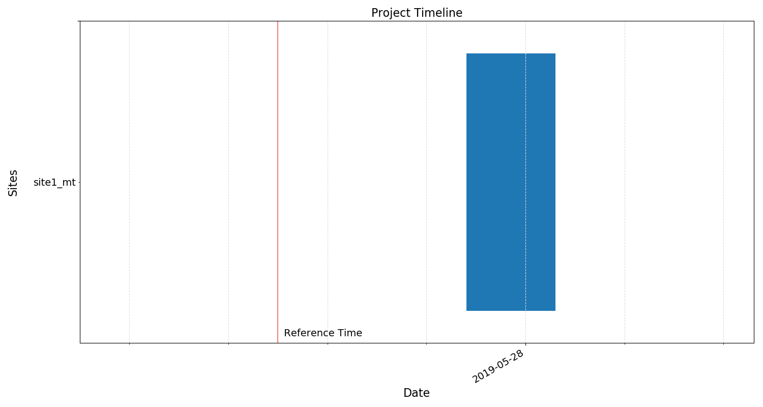
Project timeline
Time data can be viewed in the usual way in the project environment using the viewTime() method.
18 19 20 21 22 23 24 25 26 27 28 29 | # view time
from resistics.project.time import viewTime
fig = viewTime(
proj,
startDate="2019-05-27 14:15:00",
endDate="2019-05-27 15:00:00",
filter={"lpfilt": 4},
save=False,
show=False,
)
fig.savefig(imagePath / "viewTime.png")
|
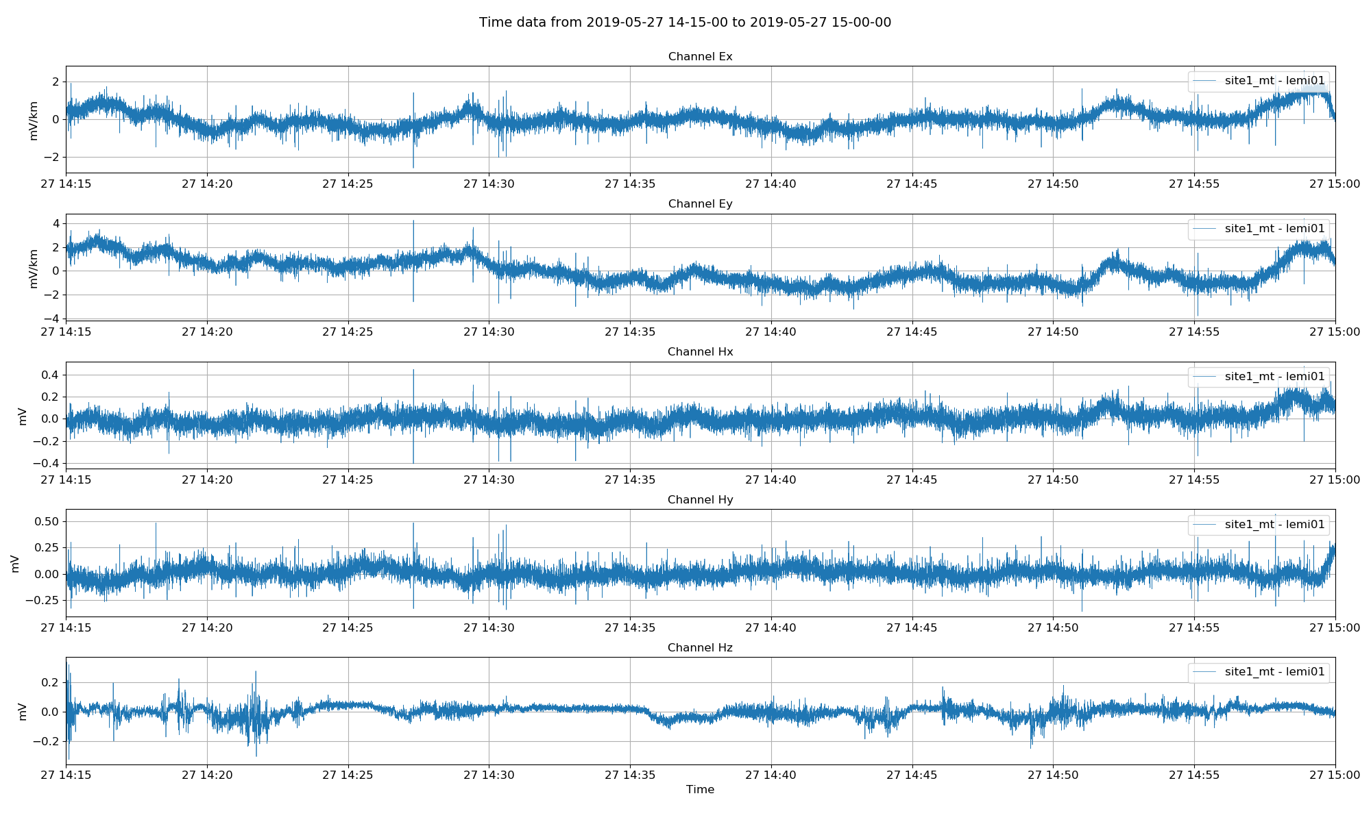
Lemi B423 magnetotelluric data in field units (mV/km for electric channels and mV ffor magnetic channels)
Next, process the data to estimate the impedance tensor. This involves calculating spectra and then doing the robust regression. Additionally, statistics are being calculated for future use.
31 32 33 34 35 36 37 38 39 40 41 42 43 44 45 | from resistics.project.spectra import calculateSpectra
from resistics.project.statistics import calculateStatistics
from resistics.project.transfunc import processProject, viewImpedance
from resistics.common.plot import plotOptionsTransferFunction, getPaperFonts
calculateSpectra(proj)
proj.refresh()
calculateStatistics(proj)
processProject(proj)
plotOptions = plotOptionsTransferFunction(figsize=(24, 12), plotfonts=getPaperFonts())
plotOptions["res_ylim"] = [1, 1000000]
figs = viewImpedance(
proj, oneplot=False, plotoptions=plotOptions, show=False, save=False
)
figs[0].savefig(imagePath / "impedance_default.png")
|
The resultant impedance tensor estimate is shown below.
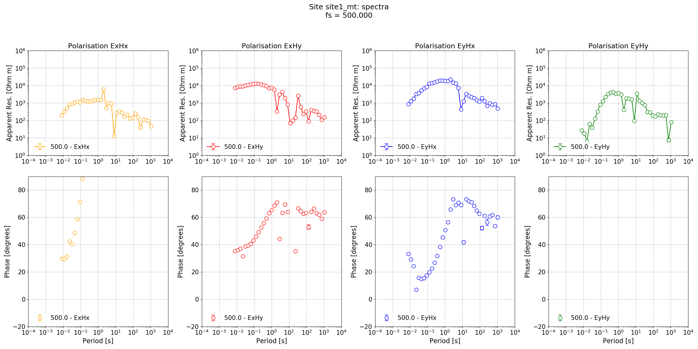
Impedance tensor estimate for Lemi B423 data at a sampling frequency of 500 Hz.
Looking at the impedance tensor estimate, there are two issues:
Dead band data looks poor, probably because of signal to noise ratio
Long period data is poor, probably due to too few windows
To deal with the second point, define a new configuration setup that will provide more windows at long periods and redo the processing. Now that because the windowing scheme has changed, a new set of spectra and statistics will need to be calculated.
1 2 3 4 5 6 7 8 9 10 11 | name = customwin
[Spectra]
specdir = "customwin"
[Window]
windowsizes = 1024, 512, 256, 256, 128, 128, 128
overlapsizes = 256, 128, 64, 64, 32, 32, 32
[Statistics]
stats = "coherence", "transferFunction",
|
1 2 3 4 5 6 7 8 9 10 11 12 13 14 15 16 17 18 19 20 21 | from datapaths import projectPath, imagePath
from resistics.project.io import loadProject
proj = loadProject(projectPath, "customconfig.ini")
proj.printInfo()
from resistics.project.spectra import calculateSpectra
from resistics.project.statistics import calculateStatistics
from resistics.project.transfunc import processProject, viewImpedance
from resistics.common.plot import plotOptionsTransferFunction, getPaperFonts
calculateSpectra(proj)
proj.refresh()
calculateStatistics(proj)
processProject(proj)
plotOptions = plotOptionsTransferFunction(figsize=(24, 12), plotfonts=getPaperFonts())
plotOptions["res_ylim"] = [1, 1000000]
figs = viewImpedance(
proj, oneplot=False, plotoptions=plotOptions, show=False, save=False
)
figs[0].savefig(imagePath / "impedance_config.png")
|
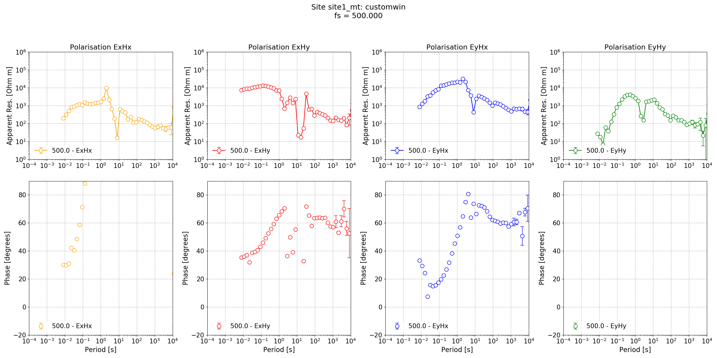
Impedance tensor estimate for Lemi B423 data at a sampling frequency of 500 Hz with a different windowing scheme
The new windowing scheme, which reduces the window size at the long periods has produced a better result at long periods. However, there has been no improvement in the dead band. For that, a coherence mask can be tried.
23 24 25 26 27 28 29 30 31 32 33 34 35 36 37 38 39 40 41 42 43 44 45 46 47 48 49 50 51 52 53 54 55 56 57 58 59 60 61 62 | # now try again with some statistics for the dead band
from resistics.project.mask import newMaskData, calculateMask
maskData = newMaskData(proj, 500)
maskData.setStats(["coherence"])
maskData.addConstraintLevel(
"coherence", {"cohExHy": [0.8, 1.0], "cohEyHx": [0.8, 1.0]}, 0
)
maskData.addConstraintLevel(
"coherence", {"cohExHy": [0.8, 1.0], "cohEyHx": [0.8, 1.0]}, 1
)
maskData.addConstraintLevel(
"coherence", {"cohExHy": [0.7, 1.0], "cohEyHx": [0.7, 1.0]}, 2
)
maskData.addConstraintLevel(
"coherence", {"cohExHy": [0.6, 1.0], "cohEyHx": [0.6, 1.0]}, 3
)
maskData.addConstraintLevel(
"coherence", {"cohExHy": [0.5, 1.0], "cohEyHx": [0.5, 1.0]}, 4
)
maskData.addConstraintLevel(
"coherence", {"cohExHy": [0.5, 1.0], "cohEyHx": [0.5, 1.0]}, 5
)
maskData.addConstraintLevel(
"coherence", {"cohExHy": [0.4, 1.0], "cohEyHx": [0.4, 1.0]}, 6
)
maskData.maskName = "coh80_100"
calculateMask(proj, maskData, sites=["site1_mt"])
# process the site with the mask
processProject(proj, masks={"site1_mt": "coh80_100"}, postpend="coh80_100")
figs = viewImpedance(
proj,
postpend="coh80_100",
oneplot=False,
plotoptions=plotOptions,
show=False,
save=False,
)
figs[0].savefig(imagePath / "impedance_config_masks.png")
|
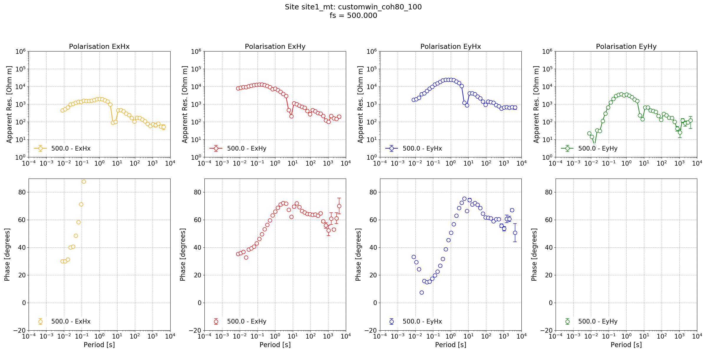
Impedance tensor estimate for Lemi B423 data at a sampling frequency of 500 Hz with a different windowing scheme and variable coherence masking for each decimation level. The result is now better than default settings in both the long periods and dead band.
The coherence mask has indeed improved the dead band reponse. With further work and investigation of statistics, it may be possible to achieve an ever better result.
Complete example scripts
For the purposes of clarity, the complete example scripts is provided below.
Creating the project.
1 2 3 4 5 6 | from datapaths import projectPath
from resistics.project.io import newProject
referenceTime = "2019-05-25 12:00:00"
proj = newProject(projectPath, referenceTime)
proj.printInfo()
|
Processing with standard parameters.
1 2 3 4 5 6 7 8 9 10 11 12 13 14 15 16 17 18 19 20 21 22 23 24 25 26 27 28 29 30 31 32 33 34 35 36 37 38 39 40 41 42 43 44 45 | from datapaths import projectPath, imagePath
from resistics.time.reader_lemib423 import folderB423Headers
# first need to create headers
sitePath = projectPath / "timeData" / "site1_mt"
folderB423Headers(
sitePath, 500, hxSensor=712, hySensor=710, hzSensor=714, hGain=16, dx=60, dy=60.7
)
# load project
from resistics.project.io import loadProject

proj = loadProject(projectPath)
proj.printInfo()
fig = proj.view()
fig.savefig(imagePath / "timeline.png")
# view time
from resistics.project.time import viewTime

fig = viewTime(
    proj,
    startDate="2019-05-27 14:15:00",
    endDate="2019-05-27 15:00:00",
    filter={"lpfilt": 4},
    save=False,
    show=False,
)
fig.savefig(imagePath / "viewTime.png")
from resistics.project.spectra import calculateSpectra
from resistics.project.statistics import calculateStatistics
from resistics.project.transfunc import processProject, viewImpedance
from resistics.common.plot import plotOptionsTransferFunction, getPaperFonts

calculateSpectra(proj)
proj.refresh()
calculateStatistics(proj)
processProject(proj)
plotOptions = plotOptionsTransferFunction(figsize=(24, 12), plotfonts=getPaperFonts())
plotOptions["res_ylim"] = [1, 1000000]
figs = viewImpedance(
    proj, oneplot=False, plotoptions=plotOptions, show=False, save=False
)
figs[0].savefig(imagePath / "impedance_default.png")
|
Processing with a configuration file.
1 2 3 4 5 6 7 8 9 10 11 12 13 14 15 16 17 18 19 20 21 22 23 24 25 26 27 28 29 30 31 32 33 34 35 36 37 38 39 40 41 42 43 44 45 46 47 48 49 50 51 52 53 54 55 56 57 58 59 60 61 62 | from datapaths import projectPath, imagePath
from resistics.project.io import loadProject
proj = loadProject(projectPath, "customconfig.ini")
proj.printInfo()
from resistics.project.spectra import calculateSpectra
from resistics.project.statistics import calculateStatistics
from resistics.project.transfunc import processProject, viewImpedance
from resistics.common.plot import plotOptionsTransferFunction, getPaperFonts
calculateSpectra(proj)
proj.refresh()
calculateStatistics(proj)
processProject(proj)
plotOptions = plotOptionsTransferFunction(figsize=(24, 12), plotfonts=getPaperFonts())
plotOptions["res_ylim"] = [1, 1000000]
figs = viewImpedance(
proj, oneplot=False, plotoptions=plotOptions, show=False, save=False
)
figs[0].savefig(imagePath / "impedance_config.png")
# now try again with some statistics for the dead band
from resistics.project.mask import newMaskData, calculateMask

maskData = newMaskData(proj, 500)
maskData.setStats(["coherence"])
maskData.addConstraintLevel(
    "coherence", {"cohExHy": [0.8, 1.0], "cohEyHx": [0.8, 1.0]}, 0
)
maskData.addConstraintLevel(
    "coherence", {"cohExHy": [0.8, 1.0], "cohEyHx": [0.8, 1.0]}, 1
)
maskData.addConstraintLevel(
    "coherence", {"cohExHy": [0.7, 1.0], "cohEyHx": [0.7, 1.0]}, 2
)
maskData.addConstraintLevel(
    "coherence", {"cohExHy": [0.6, 1.0], "cohEyHx": [0.6, 1.0]}, 3
)
maskData.addConstraintLevel(
    "coherence", {"cohExHy": [0.5, 1.0], "cohEyHx": [0.5, 1.0]}, 4
)
maskData.addConstraintLevel(
    "coherence", {"cohExHy": [0.5, 1.0], "cohEyHx": [0.5, 1.0]}, 5
)
maskData.addConstraintLevel(
    "coherence", {"cohExHy": [0.4, 1.0], "cohEyHx": [0.4, 1.0]}, 6
)
maskData.maskName = "coh80_100"
calculateMask(proj, maskData, sites=["site1_mt"])

# process the site with the mask
processProject(proj, masks={"site1_mt": "coh80_100"}, postpend="coh80_100")
figs = viewImpedance(
    proj,
    postpend="coh80_100",
    oneplot=False,
    plotoptions=plotOptions,
    show=False,
    save=False,
)
figs[0].savefig(imagePath / "impedance_config_masks.png")
|