Processing ASCII data
There are instances in which magnetotelluric time series data is better dealt with in ASCII format. ASCII format has some storage and efficiency costs, but does offer a method of last resort when either a data format is not supported or ASCII data is all that is available. To read more about the ASCII data format, see here.
The following is an example of processing long-period ASCII data from a magnotelluric observatory, recorded by a LEMI device and sampled at 0.5 Hz.
There are five data files, one for each channel:
bxnT.ascii
bynT.ascii
bznT.ascii
exmuVm.ascii
eymuVm.ascii
Note
The data files can be downloaded from here for those interested in following along.
The units of the data are the following:
Magnetic fields are in nT, which is the unit required by resistics (after calibration).
Electric fields are in microvolts per metre, which is the equivalent of mV/km, again the unit required by resistics.
To begin, a new project and site is created.
1 2 3 4 5 6 7 8 9 10 11 | from datapaths import projectPath # import the project path
from resistics.project.io import newProject
# define reference time for project
referenceTime = "2018-01-01 00:00:00"
# create a new project and print infomation
projData = newProject(projectPath, referenceTime)
projData.printInfo()
# create a new site
projData.createSite("site1")
projData.printInfo()
|
This is a single site, therefore, the reference time is of little significance. A dummy reference time has been set for the data.
Under the site directory, a time series measurement directory needs to be created. This is a simple job of making a new directory, in this case named “meas”. The data files should be copied into this directory as shown below.
asciiProject
├── calData
├── timeData
│   └── site1
|       └── meas
|           |── bxnT.ascii
|           |── bynT.ascii
|           |── bznT.ascii
|           |── exmuVm.ascii
|           └── eymuVm.ascii
├── specData
├── statData
├── maskData
├── transFuncData
├── images
└── mtProj.prj
After the project, site and measurement directory have been created, the data has to be prepared to be read in by resistics. This is achieved by using the writeTemplateHeaderFiles() method of the class TimeWriter.
1 2 3 4 5 6 7 8 9 10 11 12 13 14 15 16 17 | from datapaths import projectPath
from resistics.time.writer import TimeWriter
asciiPath = projectPath / "timeData" / "site1" / "meas"
writer = TimeWriter()
writer.setOutPath(asciiPath)
chan2FileMap = {
"Ex": "exmuVm.ascii",
"Ey": "eymuVm.ascii",
"Hx": "bxnT.ascii",
"Hy": "bynT.ascii",
"Hz": "bznT.ascii",
}
startDate = "2018-01-01 12:00:00"
writer.writeTemplateHeaderFiles(
["Ex", "Ey", "Hx", "Hy", "Hz"], chan2FileMap, 0.5, 430000, startDate
)
|
The writeTemplateHeaderFiles() creates dummy header files for the ASCII data allowing resistics to read it in appropriately. The dummy files it creates are:
chan_00.hdr
chan_01.hdr
chan_02.hdr
chan_03.hdr
chan_04.hdr
global.hdr
The measurement directory should now look like this:
asciiProject
├── calData
├── timeData
│   └── site1
|       └── meas
|           |── global.hdr
|           |── chan_00.hdr
|           |── chan_01.hdr
|           |── chan_02.hdr
|           |── chan_03.hdr
|           |── chan_04.hdr
|           |── bxnT.ascii
|           |── bynT.ascii
|           |── bznT.ascii
|           |── exmuVm.ascii
|           └── eymuVm.ascii
├── specData
├── statData
├── maskData
├── transFuncData
├── images
└── mtProj.prj
Note
For a more in depth look at what is being done here, refer to ASCII time series, which uses the same files to demonstrate ASCII data support in resistics.
The time series is now ready to be read in. In the below code block, the project and site timelines are plotted, giving two images, and then the time series is visualised.
1 2 3 4 5 6 7 8 9 10 11 12 13 14 15 16 17 18 19 20 21 22 23 24 25 | from datapaths import projectPath, imagePath
from resistics.project.io import loadProject
# load the project
projData = loadProject(projectPath)
fig = projData.view()
fig.savefig(imagePath / "projectTimeline")
# view site data
siteData = projData.getSiteData("site1")
fig = siteData.view()
fig.savefig(imagePath / "siteTimeline")
from resistics.project.time import viewTime
from resistics.common.plot import plotOptionsTime, getPaperFonts
plotOptions = plotOptionsTime(plotfonts=getPaperFonts())
fig = viewTime(
projData,
"2018-01-03 00:00:00",
"2018-01-05 00:00:00",
plotoptions=plotOptions,
save=False,
)
fig.savefig(imagePath / "viewTime")
|
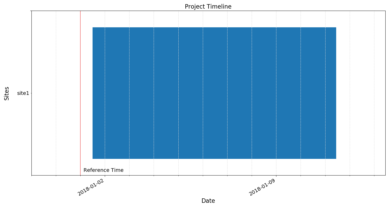
Project timeline, though the reference time is purely a dummy one.
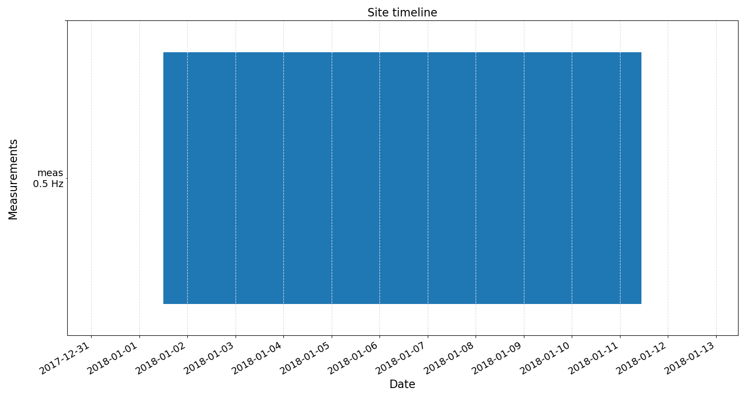
Site timeline.
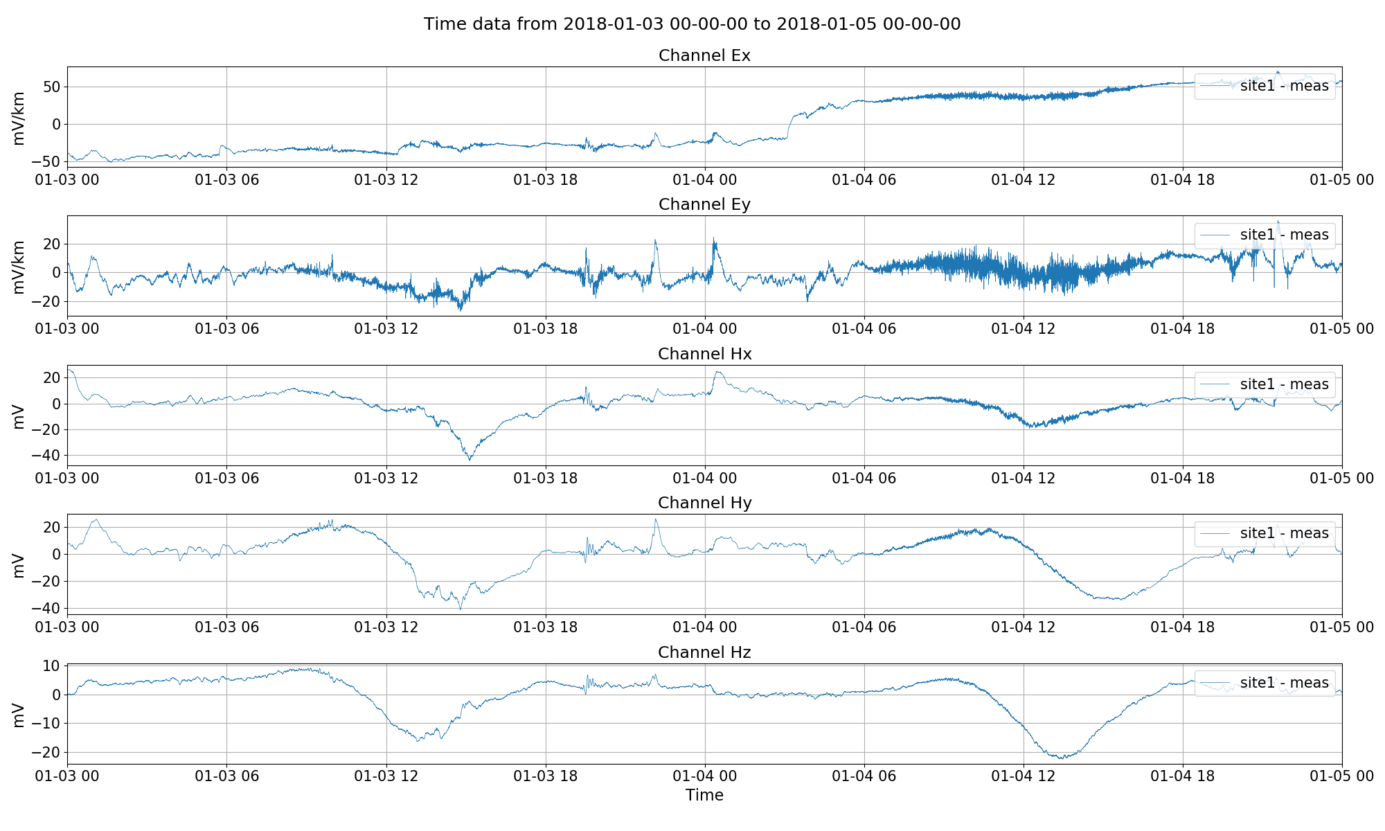
Visualising time series.
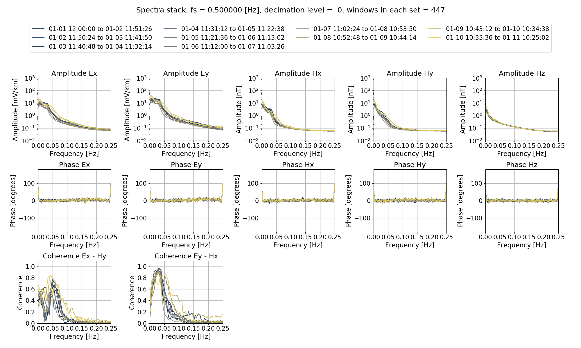
The next step is to calculate out the spectra and then produce a spectra stack plot, which will help in assessing the quality of the data.
27 28 29 30 31 32 33 34 35 36 37 38 39 40 41 42 43 44 45 46 | # calculate spectrum using standard options
from resistics.project.spectra import calculateSpectra
calculateSpectra(projData, calibrate=False)
projData.refresh()
from resistics.project.spectra import viewSpectraStack
from resistics.common.plot import plotOptionsSpec
plotOptions = plotOptionsSpec(plotfonts=getPaperFonts())
fig = viewSpectraStack(
projData,
"site1",
"meas",
coherences=[["Ex", "Hy"], ["Ey", "Hx"]],
plotoptions=plotOptions,
save=False,
show=False,
)
fig.savefig(imagePath / "viewSpectraStack")
|
The spectra stack is shown below:
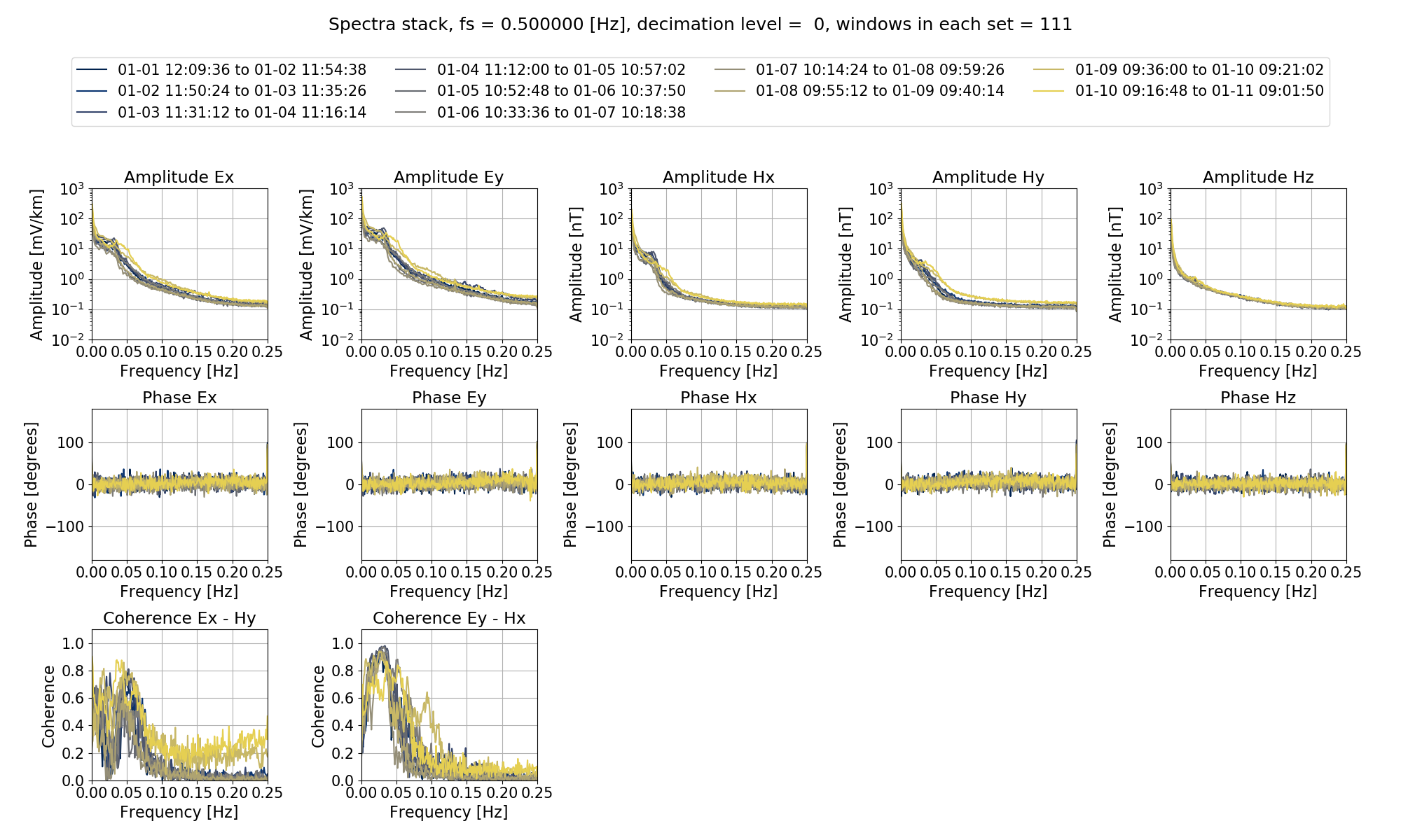
The spectra stack.
The easiest way to process the ascii data is using the default parameterisation, much like in Up and running.
48 49 50 51 52 53 54 55 56 57 58 59 60 61 62 63 64 65 66 67 68 | # process the spectra to estimate the transfer function
from resistics.project.transfunc import processProject
processProject(projData, outchans=["Ex", "Ey"])
# plot impedance tensor and save the plot
from resistics.project.transfunc import viewImpedance
from resistics.common.plot import plotOptionsTransferFunction
plotoptions = plotOptionsTransferFunction(plotfonts=getPaperFonts())
plotoptions["xlim"] = [0.01, 1000000]
plotoptions["phase_ylim"] = [-360, 360]
figs = viewImpedance(
projData,
sites=["site1"],
oneplot=True,
polarisations=["ExHy", "EyHx"],
plotoptions=plotoptions,
save=False,
)
figs[0].savefig(imagePath / "impedance_default")
|
This gives the below impedance tensor estimate.
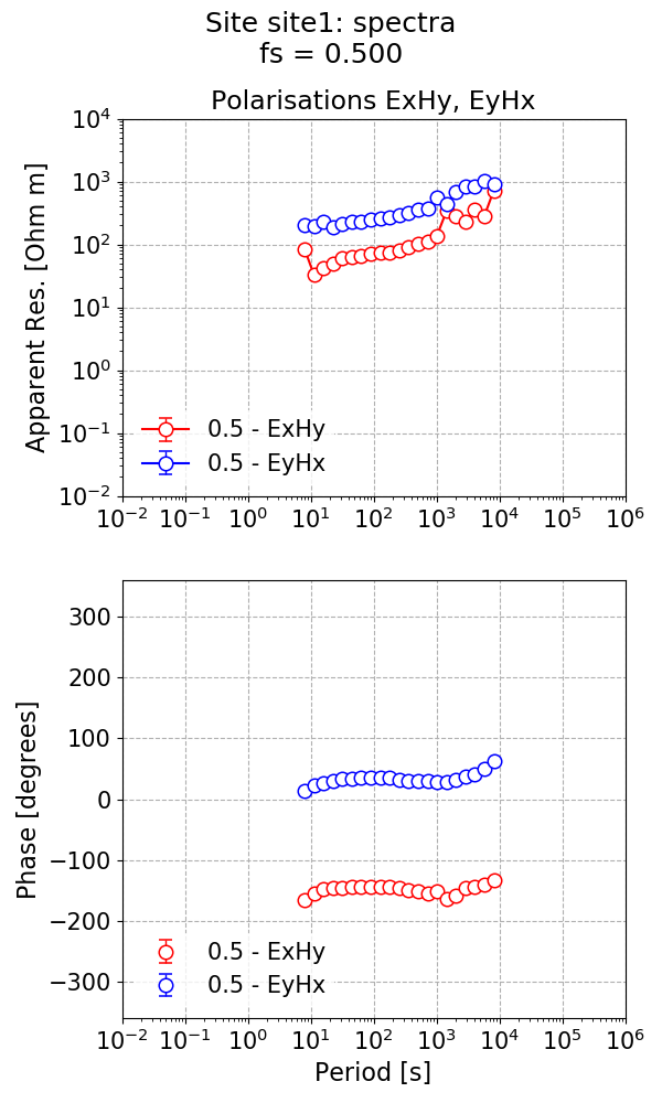
The impedance tensor estimate.
Looking at the phase estimates, the phase for the ExHy component is in the wrong quadrant. This is generally due to a different polarity convention, which can be fixed by performing a polarity reversal, which is shown below.
Note
A polarity reversal sounds impressive but is simply a multiplication by -1. This does not change impedance tensor magnitude (therefore the apparent resistivity) but will have an impact on the phase.
70 71 72 73 74 75 76 77 78 79 80 81 82 | # calculate the tipper
processProject(projData, outchans=["Ex", "Ey", "Hz"], postpend="withHz")
# plot the tipper
from resistics.project.transfunc import viewTipper
from resistics.common.plot import plotOptionsTipper
plotoptions = plotOptionsTipper(plotfonts=getPaperFonts())
plotoptions["xlim"] = [0.01, 1000000]
figs = viewTipper(
projData, sites=["site1"], postpend="withHz", plotoptions=plotoptions, save=True
)
figs[0].savefig(imagePath / "impedance_default_withHz")
|
The tipper estimate is shown below.
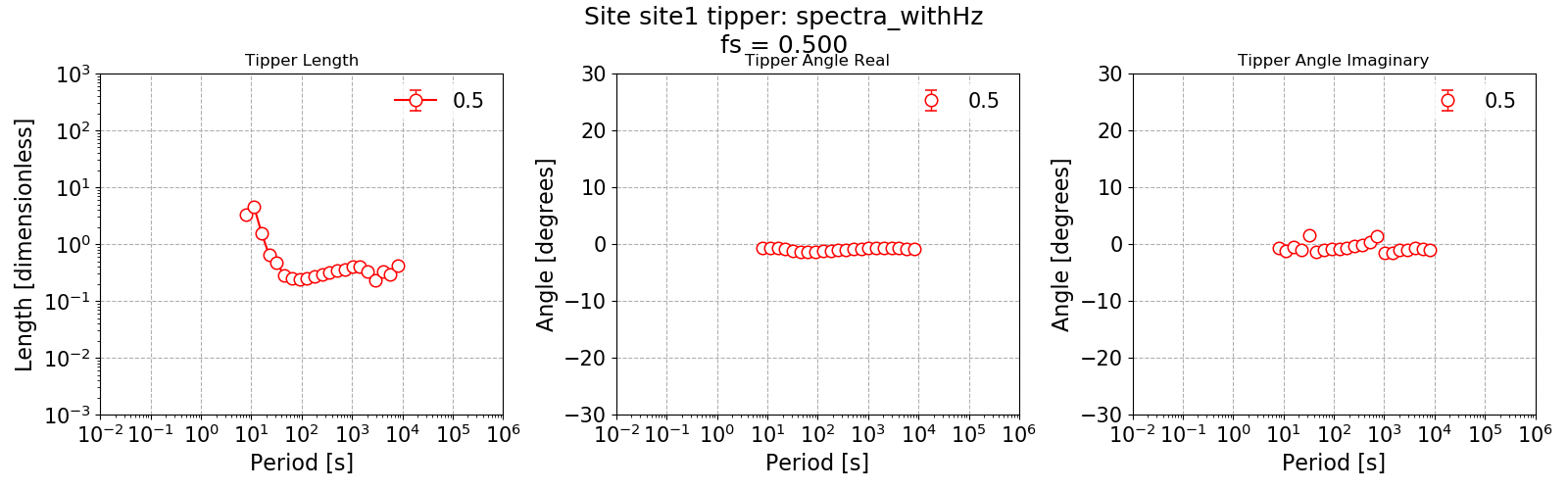
The tipper estimate.
Changing the default parameters
As described in the Using configuration files section in the Tutorial, configuration files can be used to change the default parameterisation. The default parameters are not necessarily ideal for long period MT stations sampled at low sampling frequencies (here, 0.5 Hz). Therefore, it could be sensible to change the parameters here.
A new configuration file has been made and is included below:
1 2 3 4 5 6 7 8 9 10 11 12 13 14 15 | name = dec8_5
[Spectra]
specdir = "dec8_5"
[Decimation]
numlevels = 8
[Frequencies]
perlevel = 5
[Window]
windowfactor = 2
minwindowsize = 128
minoverlapsize = 32
|
To use the configuration file, the project needs to be loaded along with the configuration file.
1 2 3 4 5 6 | from datapaths import projectPath, imagePath
from resistics.project.io import loadProject
# load the project and also provide a config file
projData = loadProject(projectPath, configFile="asciiconfig.ini")
projData.printInfo()
|
Note
As the new configuration file includes new windowing parameters, a new set of spectra will be calculated out. The specdir option in the configuration deals with this.
The first task it to view the time series data with a polarity reversal. This can be done by specifying the polreverse keyword for viewTime() as demonstrated below.
8 9 10 11 12 13 14 15 16 17 18 19 20 | from resistics.project.time import viewTime
from resistics.common.plot import plotOptionsTime, getPaperFonts
plotOptions = plotOptionsTime(plotfonts=getPaperFonts())
fig = viewTime(
projData,
"2018-01-03 00:00:00",
"2018-01-05 00:00:00",
polreverse={"Hy": True},
plotoptions=plotOptions,
save=False,
)
fig.savefig(imagePath / "viewTime_polreverse")
|

Visualising time series with Hy multiplied by -1.
Following a similar scheme as the default example, the spectra can be calculated and a spectra stack plotted. However, the polarity reversal needs to be specified when calculating the spectra, as is done in the below example.
22 23 24 25 26 27 28 29 30 31 32 33 34 35 36 37 38 39 40 41 42 | # calculate spectrum using the new configuration
from resistics.project.spectra import calculateSpectra
calculateSpectra(projData, calibrate=False, polreverse={"Hy": True})
projData.refresh()
# plot spectra stack
from resistics.project.spectra import viewSpectraStack
from resistics.common.plot import plotOptionsSpec, getPaperFonts
plotOptions = plotOptionsSpec(plotfonts=getPaperFonts())
fig = viewSpectraStack(
projData,
"site1",
"meas",
coherences=[["Ex", "Hy"], ["Ey", "Hx"]],
plotoptions=plotOptions,
save=False,
show=False,
)
fig.savefig(imagePath / "viewSpectraStack_config_polreverse")
|
The spectra stack for the new configuration using 8 decimation levels and 5 evalution frequencies per level.
As this configuration has fewer samples in a window, the resolution in frequency domain will be worse in comparison to the default parameters, which is clear from the plot.
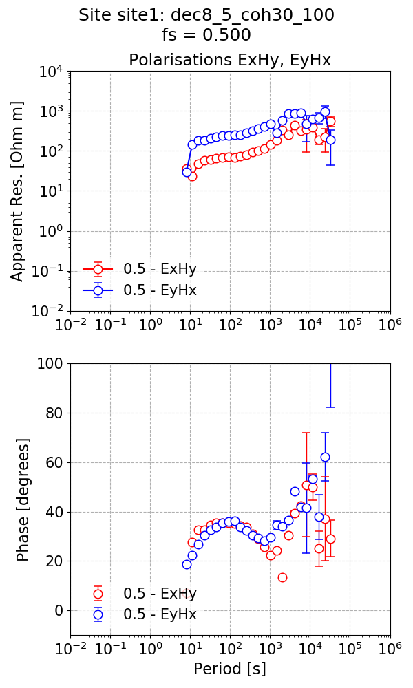
Finally, the spectra can be processed to estimate the impedance tensor and tipper. First, the impedance tensor.
44 45 46 47 48 49 50 51 52 53 54 55 56 57 58 59 60 61 62 63 64 | # calculate impedance tensor
from resistics.project.transfunc import processProject
processProject(projData, outchans=["Ex", "Ey"])
# plot impedance tensor and save the plot
from resistics.project.transfunc import viewImpedance
from resistics.common.plot import plotOptionsTransferFunction
plotoptions = plotOptionsTransferFunction(plotfonts=getPaperFonts())
plotoptions["xlim"] = [0.01, 1000000]
plotoptions["phase_ylim"] = [-10, 100]
figs = viewImpedance(
projData,
sites=["site1"],
oneplot=True,
polarisations=["ExHy", "EyHx"],
plotoptions=plotoptions,
save=True,
)
figs[0].savefig(imagePath / "impedance_config")
|
The impedance tensor estimate is shown below and now the phases are all in the correct quadrants.
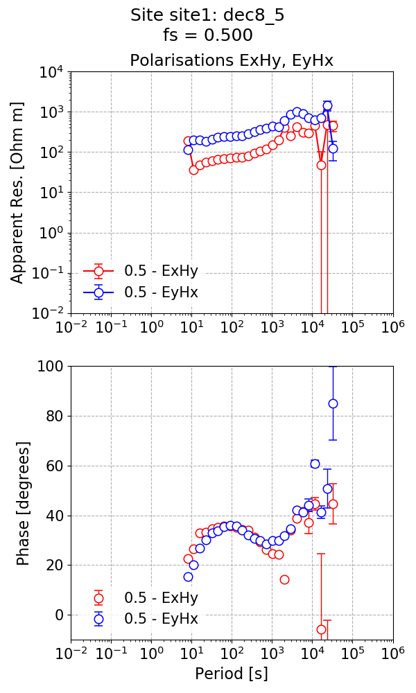
The impedance tensor estimate using 8 decimation levels and 5 evaluation frequencies per level.
And for the tipper:
66 67 68 69 70 71 72 73 74 75 76 77 | # process for the tipper
processProject(projData, outchans=["Ex", "Ey", "Hz"], postpend="withHz")
from resistics.project.transfunc import viewTipper
from resistics.common.plot import plotOptionsTipper
plotoptions = plotOptionsTipper(plotfonts=getPaperFonts())
plotoptions["xlim"] = [0.01, 1000000]
figs = viewTipper(
projData, sites=["site1"], postpend="withHz", plotoptions=plotoptions, save=True
)
figs[0].savefig(imagePath / "impedance_config_withHz")
|
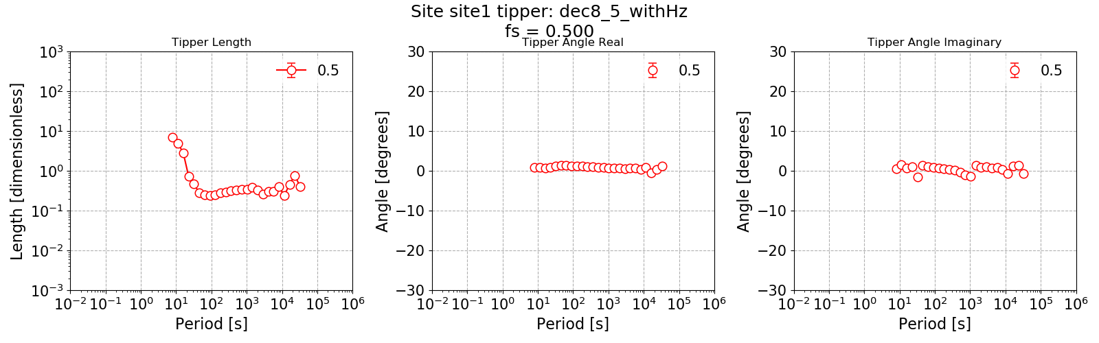
The tipper estimate using 8 decimation levels and 5 evaluation frequencies per level.
The next question to ask is whether statistics could improve the result.
Using statistics and masks
Begin once more by loading the project and configuration to continue working with the set of spectra where Hy has had a polarity reversal.
1 2 3 4 5 6 | from datapaths import projectPath, imagePath
from resistics.project.io import loadProject
# load the project and also provide a config file
projData = loadProject(projectPath, configFile="asciiconfig.ini")
projData.printInfo()
|
For more information about statistics, see the Statistics section of the tutorial. Two statistics are calculated out here: coherence and transfer function.
8 9 10 11 | # calculate statistics
from resistics.project.statistics import calculateStatistics
calculateStatistics(projData)
|
Next create a mask to perform simple coherence based rejection of time windows and view the mask.
13 14 15 16 17 18 19 20 21 22 | # create a mask based on coherence
from resistics.project.mask import newMaskData, calculateMask
maskData = newMaskData(projData, 0.5)
maskData.setStats(["coherence"])
maskData.addConstraint("coherence", {"cohExHy": [0.3, 1.0], "cohEyHx": [0.3, 1.0]})
maskData.maskName = "coh30_100"
calculateMask(projData, maskData, sites=["site1"])
fig = maskData.view(0)
fig.savefig(imagePath / "maskcoh")
|
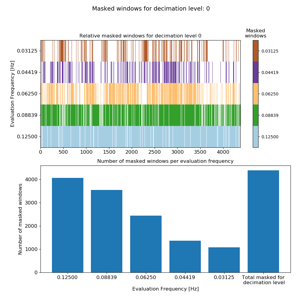
The number of masked windows for each evaluation frequency in decimation level 0.
More interesting plots can be made of statistics with masks as demonstrated in the Masks section of the tutorial, but this is left as an exercise.
Finally, calculate the impedance tensor estimate with the mask applied to exclude some windows.
24 25 26 27 28 29 30 31 32 33 34 35 36 37 38 39 40 41 42 43 44 45 46 47 | # calculate impedance tensor
from resistics.project.transfunc import processProject
processProject(
projData, outchans=["Ex", "Ey"], masks={"site1": maskData.maskName}, postpend=maskData.maskName
)
# plot transfer function and save the plot
from resistics.project.transfunc import viewImpedance
from resistics.common.plot import plotOptionsTransferFunction, getPaperFonts
plotoptions = plotOptionsTransferFunction(plotfonts=getPaperFonts())
plotoptions["xlim"] = [0.01, 1000000]
plotoptions["phase_ylim"] = [-10, 100]
figs = viewImpedance(
projData,
sites=["site1"],
postpend=maskData.maskName,
oneplot=True,
polarisations=["ExHy", "EyHx"],
plotoptions=plotoptions,
save=False,
)
figs[0].savefig(imagePath / "impedance_config_masked")
|
The impedance tensor estimate with masks applied.
If aspects of this example using ASCII data were not clear, please see the Tutorial for more information about resistics, Data formats for data supported by resistics and Advanced for an overview of the more advanced functionality of resistics.
Note, that this was not an effort to optimise the result, but rather an example and walkthrough of processing ASCII data in resistics.
Complete example scripts
For the purposes of clarity, the complete example scripts are provided below.
Create the project and a site:
1 2 3 4 5 6 7 8 9 10 11 | from datapaths import projectPath # import the project path
from resistics.project.io import newProject
# define reference time for project
referenceTime = "2018-01-01 00:00:00"
# create a new project and print infomation
projData = newProject(projectPath, referenceTime)
projData.printInfo()
# create a new site
projData.createSite("site1")
projData.printInfo()
|
Preparing the ascii data to be read in:
1 2 3 4 5 6 7 8 9 10 11 12 13 14 15 16 17 | from datapaths import projectPath
from resistics.time.writer import TimeWriter
asciiPath = projectPath / "timeData" / "site1" / "meas"
writer = TimeWriter()
writer.setOutPath(asciiPath)
chan2FileMap = {
"Ex": "exmuVm.ascii",
"Ey": "eymuVm.ascii",
"Hx": "bxnT.ascii",
"Hy": "bynT.ascii",
"Hz": "bznT.ascii",
}
startDate = "2018-01-01 12:00:00"
writer.writeTemplateHeaderFiles(
["Ex", "Ey", "Hx", "Hy", "Hz"], chan2FileMap, 0.5, 430000, startDate
)
|
Transfer function calculation with default parameters:
1 2 3 4 5 6 7 8 9 10 11 12 13 14 15 16 17 18 19 20 21 22 23 24 25 26 27 28 29 30 31 32 33 34 35 36 37 38 39 40 41 42 43 44 45 46 47 48 49 50 51 52 53 54 55 56 57 58 59 60 61 62 63 64 65 66 67 68 69 70 71 72 73 74 75 76 77 78 79 80 81 82 | from datapaths import projectPath, imagePath
from resistics.project.io import loadProject
# load the project
projData = loadProject(projectPath)
fig = projData.view()
fig.savefig(imagePath / "projectTimeline")
# view site data
siteData = projData.getSiteData("site1")
fig = siteData.view()
fig.savefig(imagePath / "siteTimeline")
from resistics.project.time import viewTime
from resistics.common.plot import plotOptionsTime, getPaperFonts
plotOptions = plotOptionsTime(plotfonts=getPaperFonts())
fig = viewTime(
projData,
"2018-01-03 00:00:00",
"2018-01-05 00:00:00",
plotoptions=plotOptions,
save=False,
)
fig.savefig(imagePath / "viewTime")
# calculate spectrum using standard options
from resistics.project.spectra import calculateSpectra

calculateSpectra(projData, calibrate=False)
projData.refresh()

from resistics.project.spectra import viewSpectraStack
from resistics.common.plot import plotOptionsSpec

plotOptions = plotOptionsSpec(plotfonts=getPaperFonts())
fig = viewSpectraStack(
    projData,
    "site1",
    "meas",
    coherences=[["Ex", "Hy"], ["Ey", "Hx"]],
    plotoptions=plotOptions,
    save=False,
    show=False,
)
fig.savefig(imagePath / "viewSpectraStack")
# process the spectra to estimate the transfer function
from resistics.project.transfunc import processProject

processProject(projData, outchans=["Ex", "Ey"])

# plot impedance tensor and save the plot
from resistics.project.transfunc import viewImpedance
from resistics.common.plot import plotOptionsTransferFunction

plotoptions = plotOptionsTransferFunction(plotfonts=getPaperFonts())
plotoptions["xlim"] = [0.01, 1000000]
plotoptions["phase_ylim"] = [-360, 360]
figs = viewImpedance(
    projData,
    sites=["site1"],
    oneplot=True,
    polarisations=["ExHy", "EyHx"],
    plotoptions=plotoptions,
    save=False,
)
figs[0].savefig(imagePath / "impedance_default")
# calculate the tipper
processProject(projData, outchans=["Ex", "Ey", "Hz"], postpend="withHz")

# plot the tipper
from resistics.project.transfunc import viewTipper
from resistics.common.plot import plotOptionsTipper

plotoptions = plotOptionsTipper(plotfonts=getPaperFonts())
plotoptions["xlim"] = [0.01, 1000000]
figs = viewTipper(
    projData, sites=["site1"], postpend="withHz", plotoptions=plotoptions, save=True
)
figs[0].savefig(imagePath / "impedance_default_withHz")
|
Run with a configuration file:
1 2 3 4 5 6 7 8 9 10 11 12 13 14 15 16 17 18 19 20 21 22 23 24 25 26 27 28 29 30 31 32 33 34 35 36 37 38 39 40 41 42 43 44 45 46 47 48 49 50 51 52 53 54 55 56 57 58 59 60 61 62 63 64 65 66 67 68 69 70 71 72 73 74 75 76 77 | from datapaths import projectPath, imagePath
from resistics.project.io import loadProject
# load the project and also provide a config file
projData = loadProject(projectPath, configFile="asciiconfig.ini")
projData.printInfo()
from resistics.project.time import viewTime
from resistics.common.plot import plotOptionsTime, getPaperFonts
plotOptions = plotOptionsTime(plotfonts=getPaperFonts())
fig = viewTime(
projData,
"2018-01-03 00:00:00",
"2018-01-05 00:00:00",
polreverse={"Hy": True},
plotoptions=plotOptions,
save=False,
)
fig.savefig(imagePath / "viewTime_polreverse")
# calculate spectrum using the new configuration
from resistics.project.spectra import calculateSpectra
calculateSpectra(projData, calibrate=False, polreverse={"Hy": True})
projData.refresh()
# plot spectra stack
from resistics.project.spectra import viewSpectraStack
from resistics.common.plot import plotOptionsSpec, getPaperFonts
plotOptions = plotOptionsSpec(plotfonts=getPaperFonts())
fig = viewSpectraStack(
projData,
"site1",
"meas",
coherences=[["Ex", "Hy"], ["Ey", "Hx"]],
plotoptions=plotOptions,
save=False,
show=False,
)
fig.savefig(imagePath / "viewSpectraStack_config_polreverse")
# calculate impedance tensor
from resistics.project.transfunc import processProject
processProject(projData, outchans=["Ex", "Ey"])
# plot impedance tensor and save the plot
from resistics.project.transfunc import viewImpedance
from resistics.common.plot import plotOptionsTransferFunction
plotoptions = plotOptionsTransferFunction(plotfonts=getPaperFonts())
plotoptions["xlim"] = [0.01, 1000000]
plotoptions["phase_ylim"] = [-10, 100]
figs = viewImpedance(
projData,
sites=["site1"],
oneplot=True,
polarisations=["ExHy", "EyHx"],
plotoptions=plotoptions,
save=True,
)
figs[0].savefig(imagePath / "impedance_config")
# process for the tipper
processProject(projData, outchans=["Ex", "Ey", "Hz"], postpend="withHz")
from resistics.project.transfunc import viewTipper
from resistics.common.plot import plotOptionsTipper
plotoptions = plotOptionsTipper(plotfonts=getPaperFonts())
plotoptions["xlim"] = [0.01, 1000000]
figs = viewTipper(
projData, sites=["site1"], postpend="withHz", plotoptions=plotoptions, save=True
)
figs[0].savefig(imagePath / "impedance_config_withHz")
|
Run with statistics:
1 2 3 4 5 6 7 8 9 10 11 12 13 14 15 16 17 18 19 20 21 22 23 24 25 26 27 28 29 30 31 32 33 34 35 36 37 38 39 40 41 42 43 44 45 46 47 | from datapaths import projectPath, imagePath
from resistics.project.io import loadProject
# load the project and also provide a config file
projData = loadProject(projectPath, configFile="asciiconfig.ini")
projData.printInfo()
# calculate statistics
from resistics.project.statistics import calculateStatistics

calculateStatistics(projData)
# create a mask based on coherence
from resistics.project.mask import newMaskData, calculateMask

maskData = newMaskData(projData, 0.5)
maskData.setStats(["coherence"])
maskData.addConstraint("coherence", {"cohExHy": [0.3, 1.0], "cohEyHx": [0.3, 1.0]})
maskData.maskName = "coh30_100"
calculateMask(projData, maskData, sites=["site1"])
fig = maskData.view(0)
fig.savefig(imagePath / "maskcoh")
# calculate impedance tensor
from resistics.project.transfunc import processProject

processProject(
    projData, outchans=["Ex", "Ey"], masks={"site1": maskData.maskName}, postpend=maskData.maskName
)

# plot transfer function and save the plot
from resistics.project.transfunc import viewImpedance
from resistics.common.plot import plotOptionsTransferFunction, getPaperFonts

plotoptions = plotOptionsTransferFunction(plotfonts=getPaperFonts())
plotoptions["xlim"] = [0.01, 1000000]
plotoptions["phase_ylim"] = [-10, 100]
figs = viewImpedance(
    projData,
    sites=["site1"],
    postpend=maskData.maskName,
    oneplot=True,
    polarisations=["ExHy", "EyHx"],
    plotoptions=plotoptions,
    save=False,
)
figs[0].savefig(imagePath / "impedance_config_masked")
|