ASCII timeseries
Resistics supports reading in of ascii data, allowing processing of data formats unsupported by resistics as long as the data can be converted into ASCII format.
ASCII data folders require a separate file for each recording channel, a global header file and header files for each channel. The data files should have extension .ascii and the header files .hdr. An example data folder for ASCII is shown below:
run1
├── global.hdr
├── chan00.hdr
├── chan01.hdr
├── chan02.hdr
├── chan03.hdr
├── chan04.hdr
├── bxnT.ascii
├── bynT.ascii
├── bznT.ascii
├── exmuVm.ascii
└── eymuVm.ascii
Note
In order for resistics to recognise an ASCII data folder, the following have to be present:
Header files with extension .hdr (global and one for each channel)
Data files with extension .ascii
Note
No scaling occurs in the ASCII data reader. All required scaling should be done prior to reading the ASCII data into resistics.
Fortunately, given some minimal information, resistics can autogenerate the header files for the ASCII data. The easiest way to explain how ASCII data works is to step through an example. To begin, there are five data files as below:
run1
├── bxnT.dat
├── bynT.dat
├── bznT.dat
├── exmuVm.dat
└── eymuVm.dat
Remember, ASCII data files need to have the extension .ascii (otherwise it would be hard to distinguish ASCII data from other formats). Therefore, the first step is to rename all the data files until the folder looks like,
run1
├── bxnT.ascii
├── bynT.ascii
├── bznT.ascii
├── exmuVm.ascii
└── eymuVm.ascii
The TimeWriter class has a handy function for autogenerating header files named writeTemplateHeaderFiles(). Its use is shown below:
1 2 3 4 5 6 7 8 9 10 11 12 13 14 15 16 17 | from datapaths import timePath, timeImages
from resistics.time.writer import TimeWriter
asciiPath = timePath / "ascii"
writer = TimeWriter()
writer.setOutPath(asciiPath)
chan2FileMap = {
"Ex": "exmuVm.ascii",
"Ey": "eymuVm.ascii",
"Hx": "bxnT.ascii",
"Hy": "bynT.ascii",
"Hz": "bznT.ascii",
}
startDate = "2018-01-01 12:00:00"
writer.writeTemplateHeaderFiles(
["Ex", "Ey", "Hx", "Hy", "Hz"], chan2FileMap, 0.5, 430000, startDate
)
|
The chan2FileMap is a dictionary that maps channel names to the actual data files. The call to writeTemplateHeaderFiles() needs to specify several parameters:
The channels as a list of strings
The map from the channel name to the data file
The sampling frequency in Hz
The number of samples
The start date of the recording
Given this information, resistics will produce a set of header files such that the data folder now looks like this:
run1
├── global.hdr
├── chan00.hdr
├── chan01.hdr
├── chan02.hdr
├── chan03.hdr
├── chan04.hdr
├── bxnT.ascii
├── bynT.ascii
├── bznT.ascii
├── exmuVm.ascii
└── eymuVm.ascii
The end time of the recording is automatically calculated given the start time, sampling frequency and number of samples. This information is inserted into the header files. The global header file contains the following information:
1 2 3 4 5 6 7 8 | HEADER = GLOBAL
sample_freq = 0.5
num_samples = 430000
start_time = 12:00:00.000000
start_date = 2018-01-01
stop_time = 10:53:18.000000
stop_date = 2018-01-11
meas_channels = 5
|
Channel metadata is stored in the channel header files. For example, the header file for channel Ex contains the following information:
1 2 3 4 5 6 7 8 9 10 11 12 13 14 15 16 17 18 19 20 21 22 23 | HEADER = CHANNEL
sample_freq = 0.5
num_samples = 430000
start_time = 12:00:00.000000
start_date = 2018-01-01
stop_time = 10:53:18.000000
stop_date = 2018-01-11
ats_data_file = exmuVm.ascii
sensor_type = None
channel_type = Ex
ts_lsb = 1
scaling_applied = True
pos_x1 = 0
pos_x2 = 1
pos_y1 = 0
pos_y2 = 1
pos_z1 = 0
pos_z2 = 1
sensor_sernum = 1
gain_stage1 = 1
gain_stage2 = 1
hchopper = 0
echopper = 0
|
The data is now ready to be read in by resistics, which is achieved with the TimeReaderAscii class.
19 20 21 22 23 | # read in ascii format
from resistics.time.reader_ascii import TimeReaderAscii
asciiReader = TimeReaderAscii(asciiPath)
asciiReader.printInfo()
|
The recording information can be printed to the terminal using the printInfo() method of all input, output handlers. An example of the output is shown below:
1 2 3 4 5 6 7 8 9 10 11 12 13 14 15 16 17 18 19 20 21 22 23 24 25 26 | 22:55:35 DataReaderAscii: ####################
22:55:35 DataReaderAscii: DATAREADERASCII INFO BEGIN
22:55:35 DataReaderAscii: ####################
22:55:35 DataReaderAscii: Data Path = timeData\ascii
22:55:35 DataReaderAscii: Global Headers
22:55:35 DataReaderAscii: {'sample_freq': 0.5, 'num_samples': 430000, 'start_time': '12:00:00.000000', 'start_date': '2018-01-01', 'stop_time': '10:53:18.000000', 'stop_date': '2018-01-11', 'meas_channels': 5}
22:55:35 DataReaderAscii: Channels found:
22:55:35 DataReaderAscii: ['Ex', 'Ey', 'Hx', 'Hy', 'Hz']
22:55:35 DataReaderAscii: Channel Map
22:55:35 DataReaderAscii: {'Ex': 0, 'Ey': 1, 'Hx': 2, 'Hy': 3, 'Hz': 4}
22:55:35 DataReaderAscii: Channel Headers
22:55:35 DataReaderAscii: Ex
22:55:35 DataReaderAscii: {'sample_freq': 0.5, 'num_samples': 430000, 'start_time': '12:00:00.000000', 'start_date': '2018-01-01', 'stop_time': '10:53:18.000000', 'stop_date': '2018-01-11', 'ats_data_file': 'exmuVm.ascii', 'sensor_type': 'None', 'channel_type': 'Ex', 'ts_lsb': 1.0, 'scaling_applied': True, 'pos_x1': 0.0, 'pos_x2': 1.0, 'pos_y1': 0.0, 'pos_y2': 1.0, 'pos_z1': 0.0, 'pos_z2': 1.0, 'sensor_sernum': 1, 'gain_stage1': 1, 'gain_stage2': 1, 'hchopper': 0, 'echopper': 0}
22:55:35 DataReaderAscii: Ey
22:55:35 DataReaderAscii: {'sample_freq': 0.5, 'num_samples': 430000, 'start_time': '12:00:00.000000', 'start_date': '2018-01-01', 'stop_time': '10:53:18.000000', 'stop_date': '2018-01-11', 'ats_data_file': 'eymuVm.ascii', 'sensor_type': 'None', 'channel_type': 'Ey', 'ts_lsb': 1.0, 'scaling_applied': True, 'pos_x1': 0.0, 'pos_x2': 1.0, 'pos_y1': 0.0, 'pos_y2': 1.0, 'pos_z1': 0.0, 'pos_z2': 1.0, 'sensor_sernum': 1, 'gain_stage1': 1, 'gain_stage2': 1, 'hchopper': 0, 'echopper': 0}
22:55:35 DataReaderAscii: Hx
22:55:35 DataReaderAscii: {'sample_freq': 0.5, 'num_samples': 430000, 'start_time': '12:00:00.000000', 'start_date': '2018-01-01', 'stop_time': '10:53:18.000000', 'stop_date': '2018-01-11', 'ats_data_file': 'bxnT.ascii', 'sensor_type': 'None', 'channel_type': 'Hx', 'ts_lsb': 1.0, 'scaling_applied': True, 'pos_x1': 0.0, 'pos_x2': 1.0, 'pos_y1': 0.0, 'pos_y2': 1.0, 'pos_z1': 0.0, 'pos_z2': 1.0, 'sensor_sernum': 1, 'gain_stage1': 1, 'gain_stage2': 1, 'hchopper': 0, 'echopper': 0}
22:55:35 DataReaderAscii: Hy
22:55:35 DataReaderAscii: {'sample_freq': 0.5, 'num_samples': 430000, 'start_time': '12:00:00.000000', 'start_date': '2018-01-01', 'stop_time': '10:53:18.000000', 'stop_date': '2018-01-11', 'ats_data_file': 'bynT.ascii', 'sensor_type': 'None', 'channel_type': 'Hy', 'ts_lsb': 1.0, 'scaling_applied': True, 'pos_x1': 0.0, 'pos_x2': 1.0, 'pos_y1': 0.0, 'pos_y2': 1.0, 'pos_z1': 0.0, 'pos_z2': 1.0, 'sensor_sernum': 1, 'gain_stage1': 1, 'gain_stage2': 1, 'hchopper': 0, 'echopper': 0}
22:55:35 DataReaderAscii: Hz
22:55:35 DataReaderAscii: {'sample_freq': 0.5, 'num_samples': 430000, 'start_time': '12:00:00.000000', 'start_date': '2018-01-01', 'stop_time': '10:53:18.000000', 'stop_date': '2018-01-11', 'ats_data_file': 'bznT.ascii', 'sensor_type': 'None', 'channel_type': 'Hz', 'ts_lsb': 1.0, 'scaling_applied': True, 'pos_x1': 0.0, 'pos_x2': 1.0, 'pos_y1': 0.0, 'pos_y2': 1.0, 'pos_z1': 0.0, 'pos_z2': 1.0, 'sensor_sernum': 1, 'gain_stage1': 1, 'gain_stage2': 1, 'hchopper': 0, 'echopper': 0}
22:55:35 DataReaderAscii: Note: Field units used. Physical data has units mV/km for electric fields and mV for magnetic fields
22:55:35 DataReaderAscii: Note: To get magnetic field in nT, please calibrate
22:55:35 DataReaderAscii: ####################
22:55:35 DataReaderAscii: DATAREADERASCII INFO END
22:55:35 DataReaderAscii: ####################
|
The next step is to read some data and plot it. Resistics does not load the data into memory until it is requested. Further, the package only reads the requested data. The full dataset can be read by using the getPhysicalSamples() method. Note again that no scaling is applied anywhere for ASCII data and getPhysicalSamples() will return the same result as getUnscaledSamples(). Both of these return a TimeData object.
25 26 27 28 29 30 31 32 33 34 | # get data and view
import matplotlib.pyplot as plt
asciiData = asciiReader.getPhysicalSamples()
asciiData.printInfo()
fig = plt.figure(figsize=(16, 3 * asciiData.numChans))
asciiData.view(fig=fig, label="ASCII format", legend=True)
fig.tight_layout(rect=[0, 0.02, 1, 0.96])
plt.show()
fig.savefig(timeImages / "ascii.png")
|
asciiData.printInfo() prints time data information to the terminal. An alternative way to do this is to simply print(asciiData).
1 2 3 4 5 6 7 8 9 10 11 12 13 14 15 16 17 | 22:55:38 TimeData: ####################
22:55:38 TimeData: TIMEDATA INFO BEGIN
22:55:38 TimeData: ####################
22:55:38 TimeData: Sampling frequency [Hz] = 0.5
22:55:38 TimeData: Sample rate [s] = 2.0
22:55:38 TimeData: Number of samples = 430000
22:55:38 TimeData: Number of channels = 5
22:55:38 TimeData: Channels = ['Ex', 'Ey', 'Hx', 'Hy', 'Hz']
22:55:38 TimeData: Start time = 2018-01-01 12:00:00
22:55:38 TimeData: Stop time = 2018-01-11 10:53:18
22:55:38 TimeData: Comments
22:55:38 TimeData: Unscaled data 2018-01-01 12:00:00 to 2018-01-11 10:53:18 read in from measurement timeData\ascii, samples 0 to 429999
22:55:38 TimeData: Sampling frequency 0.5
22:55:38 TimeData: Remove zeros: False, remove nans: False, remove average: True
22:55:38 TimeData: ####################
22:55:38 TimeData: TIMEDATA INFO END
22:55:38 TimeData: ####################
|
Time data can be plotted by using the class view() method. By passing a matplotlib figure to this, the layout can be controlled as required. The resulting image is:
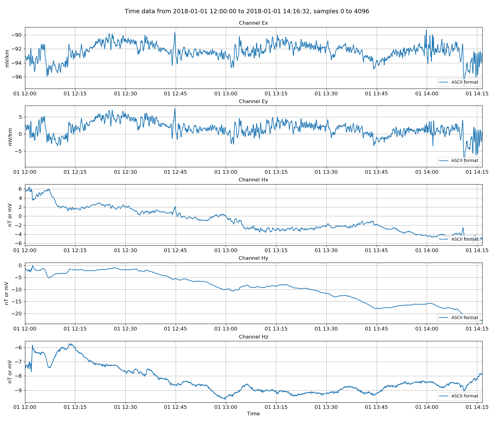
Viewing ASCII data
Ascii time data objects are like any other time data objects returned by the other data readers. The time data object can be written out in the internal binary format to increase reading speed and reduce storage cost. This can be done with the TimeWriterInternal class.
36 37 38 39 40 41 42 | # now write out as internal format
from resistics.time.writer_internal import TimeWriterInternal
ascii_2intenrnal = timePath / "asciiInternal"
writer = TimeWriterInternal()
writer.setOutPath(ascii_2intenrnal)
writer.writeDataset(asciiReader, physical=True)
|
This dataset will be written out with a comments file that tracks the history of the data. For this example, the comments file looks like:
1 2 3 4 5 | Unscaled data 2018-01-01 12:00:00 to 2018-01-11 10:53:18 read in from measurement E:\magnetotellurics\code\resisticsdata\formats\timeData\ascii, samples 0 to 429999
Sampling frequency 0.5
Remove zeros: False, remove nans: False, remove average: True
Time series dataset written to E:\magnetotellurics\code\resisticsdata\formats\timeData\asciiInternal on 2019-10-05 18:08:36.041289 using resistics 0.0.6.dev2
---------------------------------------------------
|
To validate the output against the input, the internally formatted data can be read back in using the TimeReaderInternal class and compared to the original ASCII data.
44 45 46 47 48 49 50 51 52 53 54 55 56 57 58 59 | # read in internal format
from resistics.time.reader_internal import TimeReaderInternal
internalReader = TimeReaderInternal(ascii_2intenrnal)
internalReader.printInfo()
internalReader.printComments()
internalData = internalReader.getPhysicalSamples()
internalData.printInfo()
# now plot the two datasets together
fig = plt.figure(figsize=(16, 3 * asciiData.numChans))
asciiData.view(fig=fig, sampleStop=500, label="ASCII format", legend=True)
internalData.view(fig=fig, sampleStop=500, label="Internal format", legend=True)
fig.tight_layout(rect=[0, 0.02, 1, 0.96])
plt.show()
fig.savefig(timeImages / "ascii_vs_internal.png")
|
Reading in the internal data is very similar to reading in the ASCII data. Another benefit of creating a figure and passing it through to the view() method is that multiple datasets can be plotted on the same figure. The final data comparison figure is shown below.
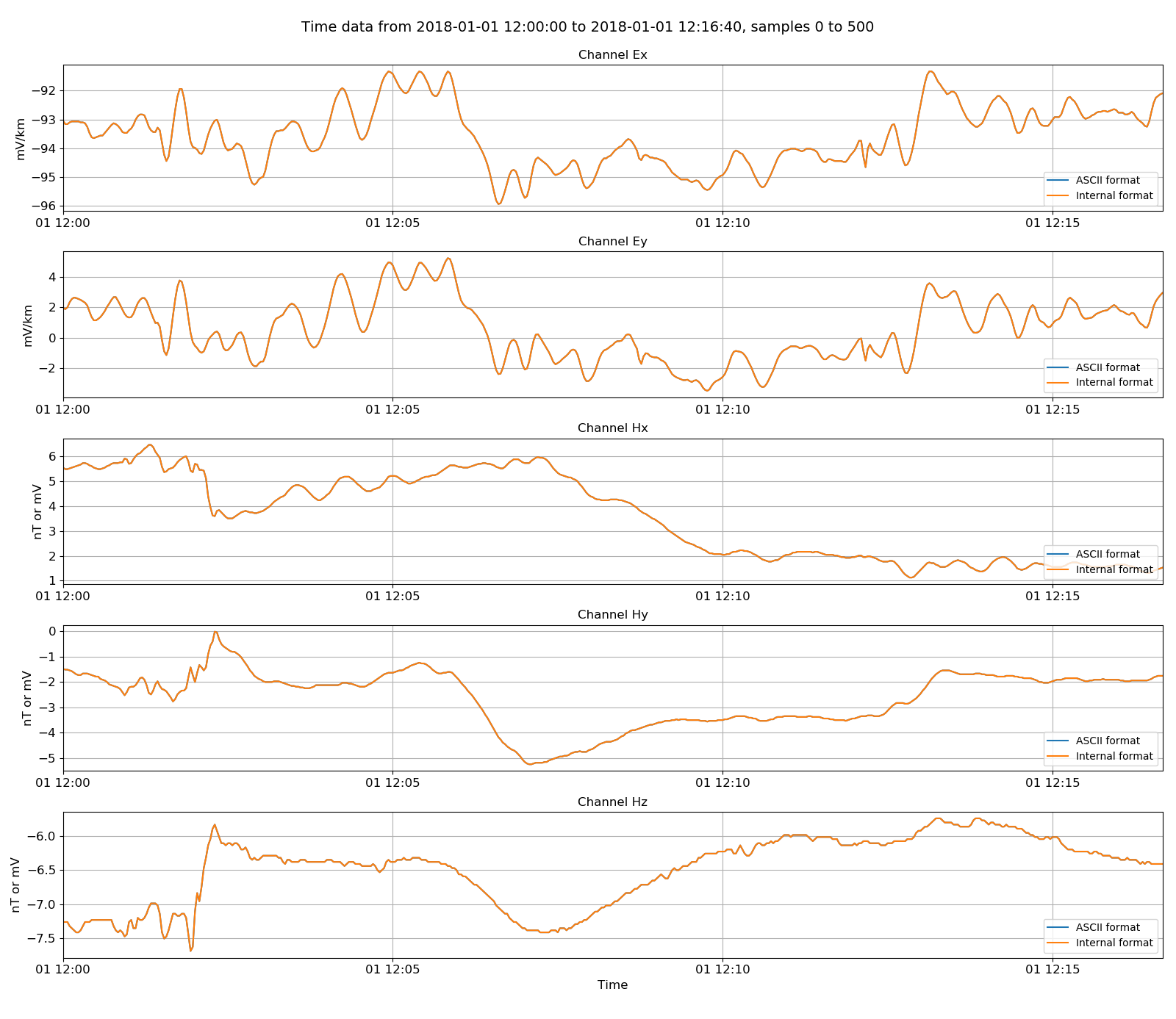
ASCII data and the binary internal format
Complete example script
For the purposes of clarity, the complete example script is shown below.
1 2 3 4 5 6 7 8 9 10 11 12 13 14 15 16 17 18 19 20 21 22 23 24 25 26 27 28 29 30 31 32 33 34 35 36 37 38 39 40 41 42 43 44 45 46 47 48 49 50 51 52 53 54 55 56 57 58 59 | from datapaths import timePath, timeImages
from resistics.time.writer import TimeWriter
asciiPath = timePath / "ascii"
writer = TimeWriter()
writer.setOutPath(asciiPath)
chan2FileMap = {
"Ex": "exmuVm.ascii",
"Ey": "eymuVm.ascii",
"Hx": "bxnT.ascii",
"Hy": "bynT.ascii",
"Hz": "bznT.ascii",
}
startDate = "2018-01-01 12:00:00"
writer.writeTemplateHeaderFiles(
["Ex", "Ey", "Hx", "Hy", "Hz"], chan2FileMap, 0.5, 430000, startDate
)
# read in ascii format
from resistics.time.reader_ascii import TimeReaderAscii

asciiReader = TimeReaderAscii(asciiPath)
asciiReader.printInfo()
# get data and view
import matplotlib.pyplot as plt

asciiData = asciiReader.getPhysicalSamples()
asciiData.printInfo()
fig = plt.figure(figsize=(16, 3 * asciiData.numChans))
asciiData.view(fig=fig, label="ASCII format", legend=True)
fig.tight_layout(rect=[0, 0.02, 1, 0.96])
plt.show()
fig.savefig(timeImages / "ascii.png")
# now write out as internal format
from resistics.time.writer_internal import TimeWriterInternal

ascii_2intenrnal = timePath / "asciiInternal"
writer = TimeWriterInternal()
writer.setOutPath(ascii_2intenrnal)
writer.writeDataset(asciiReader, physical=True)
# read in internal format
from resistics.time.reader_internal import TimeReaderInternal

internalReader = TimeReaderInternal(ascii_2intenrnal)
internalReader.printInfo()
internalReader.printComments()
internalData = internalReader.getPhysicalSamples()
internalData.printInfo()

# now plot the two datasets together
fig = plt.figure(figsize=(16, 3 * asciiData.numChans))
asciiData.view(fig=fig, sampleStop=500, label="ASCII format", legend=True)
internalData.view(fig=fig, sampleStop=500, label="Internal format", legend=True)
fig.tight_layout(rect=[0, 0.02, 1, 0.96])
plt.show()
fig.savefig(timeImages / "ascii_vs_internal.png")
|