ATS timeseries
ATS format is a one of the more straight-forward formats to support. Header files come in XML format and the data is stored in binary format with a single file for each channel. The data files have extension .ats. An example data folder for ATS is shown below:
meas_2012-02-10_11-05-00
├── 059_V01_2012-02-10_11-05-00_0.xml
├── 059_V01_C00_R000_TEx_BL_4096H.ats
├── 059_V01_C01_R000_TEy_BL_4096H.ats
├── 059_V01_C02_R000_THx_BL_4096H.ats
├── 059_V01_C02_R000_THy_BL_4096H.ats
└── 059_V01_C02_R000_THz_BL_4096H.ats
Note
In order for resistics to recognise an ATS data folder, the following have to be present:
A header file with extension .xml
Data files with extension .ats
Note
Unscaled units for ATS data are as follows:
All channels are in integer counts
ATS files are opened in resistics using the TimeReaderATS class. An example is provided below:
1 2 3 4 5 6 7 | from datapaths import timePath, timeImages
from resistics.time.reader_ats import TimeReaderATS
# read ats data
atsPath = timePath / "ats"
atsReader = TimeReaderATS(atsPath)
atsReader.printInfo()
|
atsReader.printInfo() prints the measurement information out to the terminal and displays various recording parameters.
1 2 3 4 5 6 7 8 9 10 11 12 13 14 15 16 17 18 19 20 21 22 23 24 25 26 | 14:18:00 DataReaderATS: ####################
14:18:00 DataReaderATS: DATAREADERATS INFO BEGIN
14:18:00 DataReaderATS: ####################
14:18:00 DataReaderATS: Data Path = testData\ats
14:18:00 DataReaderATS: Global Headers
14:18:00 DataReaderATS: {'start_time': '02:35:00.000000', 'start_date': '2016-02-21', 'stop_time': '06:27:12.375000', 'stop_date': '2016-02-21', 'meas_channels': 5, 'sample_freq': 128.0, 'num_samples': 1783345}
14:18:00 DataReaderATS: Channels found:
14:18:00 DataReaderATS: ['Ex', 'Ey', 'Hx', 'Hy', 'Hz']
14:18:00 DataReaderATS: Channel Map
14:18:00 DataReaderATS: {'Ex': 0, 'Ey': 1, 'Hx': 2, 'Hy': 3, 'Hz': 4}
14:18:00 DataReaderATS: Channel Headers
14:18:00 DataReaderATS: Ex
14:18:00 DataReaderATS: {'gain_stage1': 16, 'gain_stage2': 1, 'hchopper': 0, 'echopper': 0, 'start_time': '02:35:00.000000', 'start_date': '2016-02-21', 'sample_freq': 128.0, 'num_samples': 1783345, 'ats_data_file': '443_V01_C00_R001_TEx_BL_128H.ats', 'sensor_type': 'EFP06', 'channel_type': 'Ex', 'ts_lsb': -1.76666e-06, 'pos_x1': -45.0, 'pos_x2': 41.0, 'pos_y1': 0.0, 'pos_y2': 0.0, 'pos_z1': 0.0, 'pos_z2': 0.0, 'sensor_sernum': 0, 'lsb_applied': False, 'stop_date': '2016-02-21', 'stop_time': '06:27:12.375000'}
14:18:00 DataReaderATS: Ey
14:18:00 DataReaderATS: {'gain_stage1': 16, 'gain_stage2': 1, 'hchopper': 0, 'echopper': 0, 'start_time': '02:35:00.000000', 'start_date': '2016-02-21', 'sample_freq': 128.0, 'num_samples': 1783345, 'ats_data_file': '443_V01_C01_R001_TEy_BL_128H.ats', 'sensor_type': 'EFP06', 'channel_type': 'Ey', 'ts_lsb': -1.76514e-06, 'pos_x1': 0.0, 'pos_x2': 0.0, 'pos_y1': -45.0, 'pos_y2': 41.1, 'pos_z1': 0.0, 'pos_z2': 0.0, 'sensor_sernum': 0, 'lsb_applied': False, 'stop_date': '2016-02-21', 'stop_time': '06:27:12.375000'}
14:18:00 DataReaderATS: Hx
14:18:00 DataReaderATS: {'gain_stage1': 2, 'gain_stage2': 1, 'hchopper': 1, 'echopper': 0, 'start_time': '02:35:00.000000', 'start_date': '2016-02-21', 'sample_freq': 128.0, 'num_samples': 1783345, 'ats_data_file': '443_V01_C02_R001_THx_BL_128H.ats', 'sensor_type': 'MFS06e', 'channel_type': 'Hx', 'ts_lsb': -0.000112802, 'pos_x1': 0.0, 'pos_x2': 0.0, 'pos_y1': 0.0, 'pos_y2': 0.0, 'pos_z1': 0.0, 'pos_z2': 0.0, 'sensor_sernum': 612, 'lsb_applied': False, 'stop_date': '2016-02-21', 'stop_time': '06:27:12.375000'}
14:18:00 DataReaderATS: Hy
14:18:00 DataReaderATS: {'gain_stage1': 1, 'gain_stage2': 1, 'hchopper': 1, 'echopper': 0, 'start_time': '02:35:00.000000', 'start_date': '2016-02-21', 'sample_freq': 128.0, 'num_samples': 1783345, 'ats_data_file': '443_V01_C03_R001_THy_BL_128H.ats', 'sensor_type': 'MFS06e', 'channel_type': 'Hy', 'ts_lsb': -0.000225735, 'pos_x1': 0.0, 'pos_x2': 0.0, 'pos_y1': 0.0, 'pos_y2': 0.0, 'pos_z1': 0.0, 'pos_z2': 0.0, 'sensor_sernum': 613, 'lsb_applied': False, 'stop_date': '2016-02-21', 'stop_time': '06:27:12.375000'}
14:18:00 DataReaderATS: Hz
14:18:00 DataReaderATS: {'gain_stage1': 16, 'gain_stage2': 1, 'hchopper': 1, 'echopper': 0, 'start_time': '02:35:00.000000', 'start_date': '2016-02-21', 'sample_freq': 128.0, 'num_samples': 1783345, 'ats_data_file': '443_V01_C04_R001_THz_BL_128H.ats', 'sensor_type': 'MFS06e', 'channel_type': 'Hz', 'ts_lsb': -1.41103e-05, 'pos_x1': 0.0, 'pos_x2': 0.0, 'pos_y1': 0.0, 'pos_y2': 0.0, 'pos_z1': 0.0, 'pos_z2': 0.0, 'sensor_sernum': 0, 'lsb_applied': False, 'stop_date': '2016-02-21', 'stop_time': '06:27:12.375000'}
14:18:00 DataReaderATS: Note: Field units used. Physical data has units mV/km for electric fields and mV for magnetic fields
14:18:00 DataReaderATS: Note: To get magnetic field in nT, please calibrate
14:18:00 DataReaderATS: ####################
14:18:00 DataReaderATS: DATAREADERATS INFO END
14:18:00 DataReaderATS: ####################
|
This shows the headers read in by resistics and their values. There are both global headers, which apply to all the channels, and channel specific headers.
Resistics does not immediately load timeseries data into memory. In order to read the data from the files, it needs to be requested.
9 10 11 12 13 | # get unscaled data
startTime = "2016-02-21 03:00:00"
stopTime = "2016-02-21 04:00:00"
unscaledData = atsReader.getUnscaledData(startTime, stopTime)
unscaledData.printInfo()
|
atsReader.getUnscaledData(startTime, stopTime) will read timeseries data from the data files and returns a TimeData object. Unscaled data is the raw data without any conversion to field units. The units for unscaled data are not consistent between data formats and in the case of ATS data are integer counts.
After reading in some data, it is natural to view it. TimeData can be viewed using the view() method of the class. Passing a matplotlib figure object to this method allows for more control over the layout of the plot.
15 16 17 18 19 20 21 22 | # view unscaled data
import matplotlib.pyplot as plt
fig = plt.figure(figsize=(16, 3 * unscaledData.numChans))
unscaledData.view(fig=fig, sampleStop=20000)
fig.tight_layout(rect=[0, 0.02, 1, 0.96])
plt.show()
fig.savefig(timeImages / "ats_unscaledData.png")
|
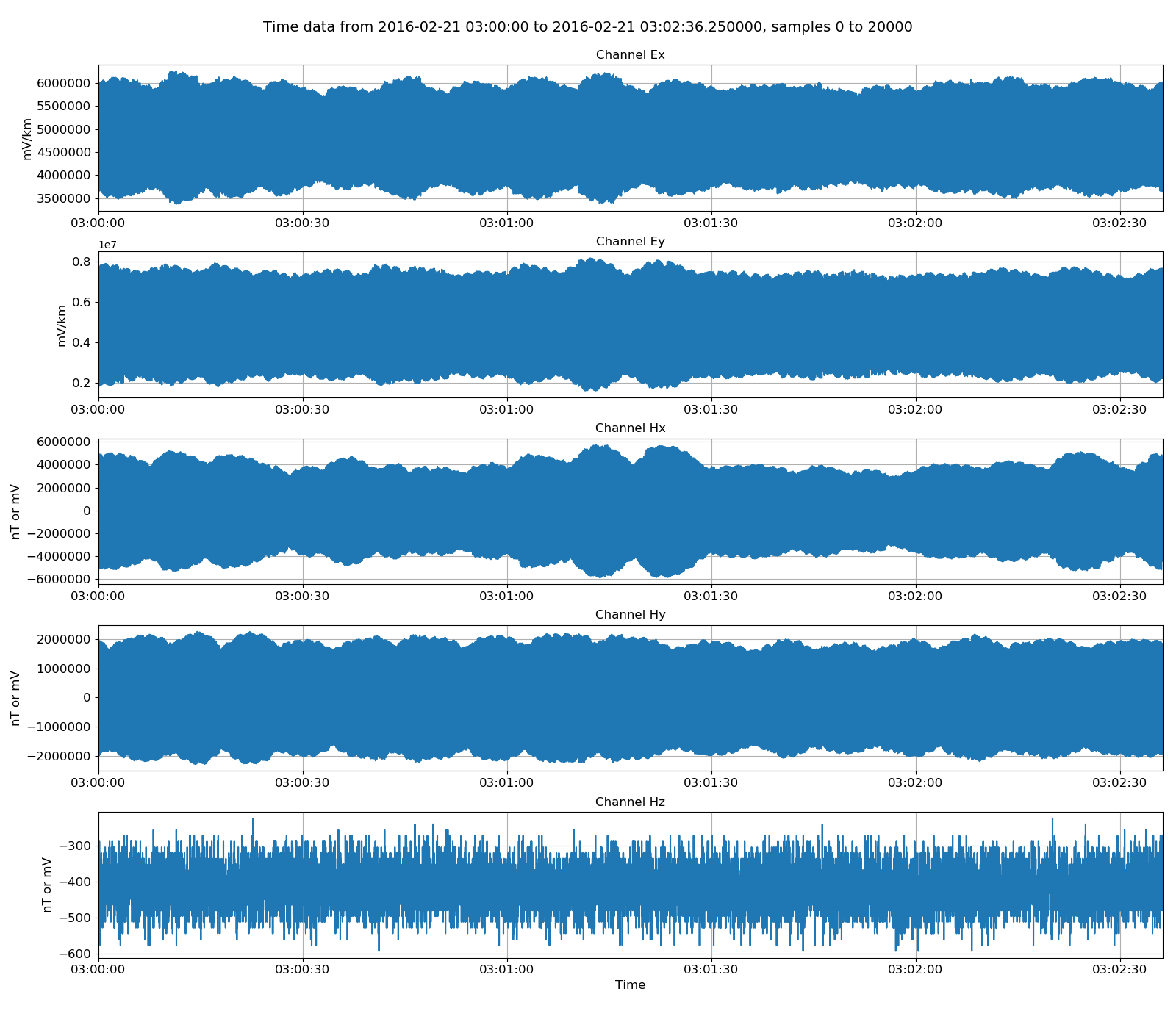
Viewing unscaled data
Physical data, which is converted to field units, can be returned by using the getPhysicalData() method. If physical data for the whole recording is required, an alternative is to use getPhysicalSamples(), which does not require specification of a start and end time.
24 25 26 27 28 29 30 31 | # get physical data, which is converted to field units
physicalATSData = atsReader.getPhysicalData(startTime, stopTime)
physicalATSData.printInfo()
fig = plt.figure(figsize=(16, 3 * physicalATSData.numChans))
fig = physicalATSData.view(fig=fig, sampleStop=20000)
fig.tight_layout(rect=[0, 0.02, 1, 0.96])
plt.show()
fig.savefig(timeImages / "ats_physicalData.png")
|
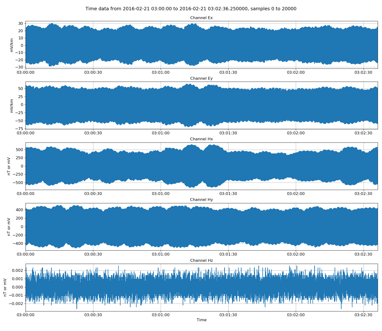
Viewing data scaled to field units
There are a few helpful methods built in to resistics for manipulating time series data. These are in time. In the example below, the time data is low pass filtered at 4Hz to remove any powerline or rail noise that might be in the data.
33 34 35 36 37 38 39 40 41 | # all we see is 50Hz and 16Hz noise - apply low pass filter
from resistics.time.filter import lowPass
filteredATSData = lowPass(physicalATSData, 4, inplace=False)
fig = plt.figure(figsize=(16, 3 * filteredATSData.numChans))
fig = filteredATSData.view(fig=fig, sampleStop=20000)
fig.tight_layout(rect=[0, 0.02, 1, 0.96])
plt.show()
fig.savefig(timeImages / "ats_filteredData.png")
|
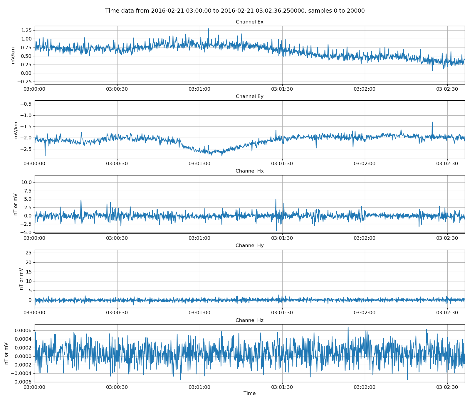
Viewing physical data low pass filtered to 4Hz
Resistics supports the writing out of data in an internal format. An examples of converting a whole dataset from ATS format to internal format is shown below.
43 44 45 46 47 48 49 | # now write out as internal format
from resistics.time.writer_internal import TimeWriterInternal
ats_2intenrnal = timePath / "atsInternal"
writer = TimeWriterInternal()
writer.setOutPath(ats_2intenrnal)
writer.writeDataset(atsReader, physical=True)
|
In nearly every case, it is best to write out data in physical format. When this is done, no further scaling will be applied when the data is read in again.
Warning
Data can be written out in unscaled format. However, each format applies different scalings when data is read in, so it is possible to write out unscaled samples in internal format and then upon reading, have it scaled incorrectly. Therefore, it is nearly always best to write out physical samples.
Writing out an internally formatted dataset will additionally write out a set of comments. These comments keep track of what has been done to the timeseries data and are there to improve repoducibility and traceability. Read more about comments here. The comments for this internally formatted dataset are:
1 2 3 4 5 6 7 8 9 10 11 12 | Unscaled data 2016-02-21 02:35:00 to 2016-02-21 06:27:12.375000 read in from measurement E:\magnetotellurics\code\resisticsdata\formats\timeData\ats, samples 0 to 1783344
Sampling frequency 128.0
Scaling channel Ex with scalar -1.76666e-06 to give mV
Dividing channel Ex by electrode distance 0.086 km to give mV/km
Scaling channel Ey with scalar -1.76514e-06 to give mV
Dividing channel Ey by electrode distance 0.0861 km to give mV/km
Scaling channel Hx with scalar -0.000112802 to give mV
Scaling channel Hy with scalar -0.000225735 to give mV
Scaling channel Hz with scalar -1.41103e-05 to give mV
Remove zeros: False, remove nans: False, remove average: True
Time series dataset written to E:\magnetotellurics\code\resisticsdata\formats\timeData\atsInternal on 2019-10-05 18:09:07.436640 using resistics 0.0.6.dev2
---------------------------------------------------
|
The internal format data can be read in and visually compared to the original data.
51 52 53 54 55 56 57 58 59 60 61 62 63 64 65 66 | # read in internal format
from resistics.time.reader_internal import TimeReaderInternal
internalReader = TimeReaderInternal(ats_2intenrnal)
internalReader.printInfo()
internalReader.printComments()
physicalInternalData = internalReader.getPhysicalData(startTime, stopTime)
physicalInternalData.printInfo()
# now plot the two datasets together
fig = plt.figure(figsize=(16, 3 * physicalATSData.numChans))
physicalATSData.view(fig=fig, sampleStop=200, label="ATS format", legend=True)
physicalInternalData.view(fig=fig, sampleStop=200, label="Internal format", legend=True)
fig.tight_layout(rect=[0, 0.02, 1, 0.96])
plt.show()
fig.savefig(timeImages / "ats_vs_internal.png")
|
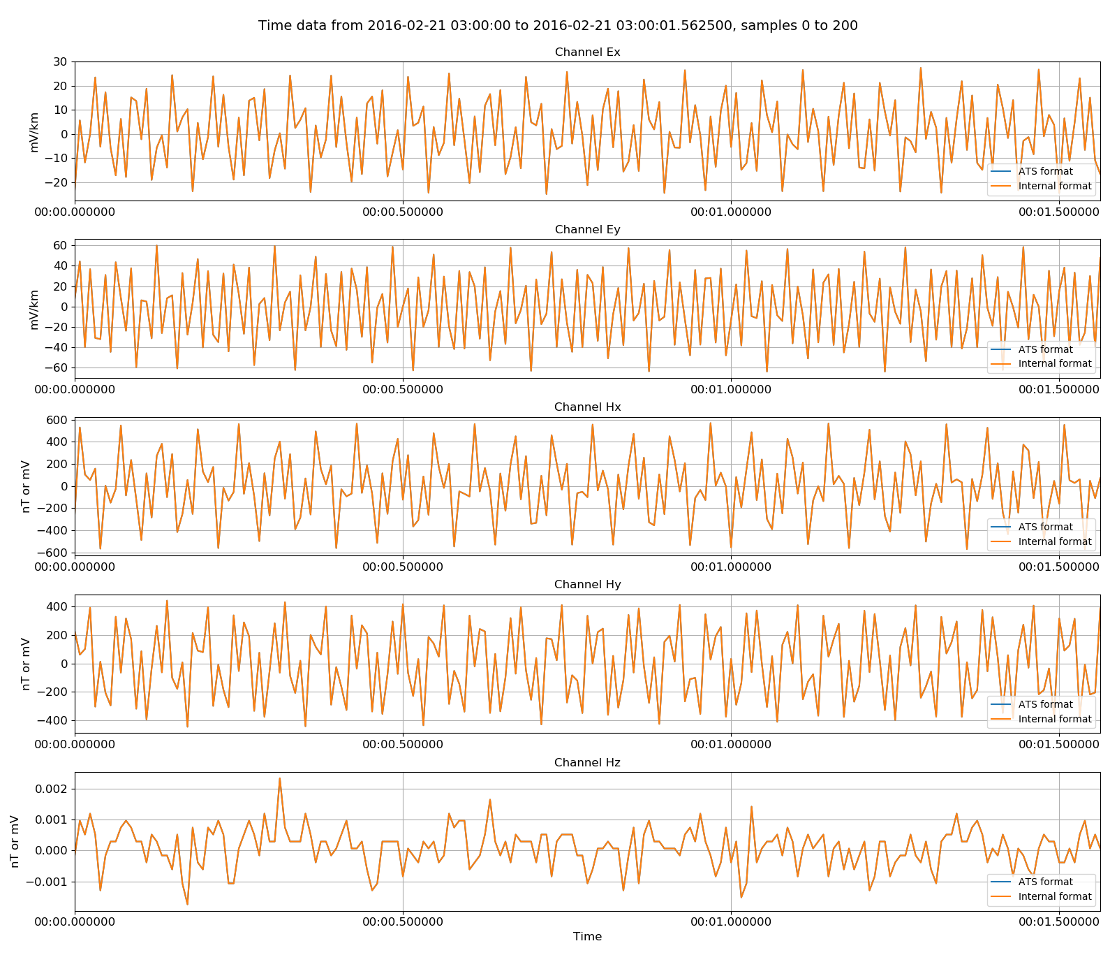
Original ATS data versus the internally formatted data
Additionally, resistics can write out data in ASCII format, which allows users to view the data values, plot them in other software or otherwise transport the data for external analysis.
68 69 70 71 72 73 74 | # now write out as ascii format
from resistics.time.writer_ascii import TimeWriterAscii
ats_2ascii = timePath / "atsAscii"
writer = TimeWriterAscii()
writer.setOutPath(ats_2ascii)
writer.writeDataset(atsReader, physical=True)
|
Again, this dataset is written out with a set of comments.
1 2 3 4 5 | Unscaled data 2018-01-01 12:00:00 to 2018-01-11 10:53:18 read in from measurement E:\magnetotellurics\code\resisticsdata\formats\timeData\ascii, samples 0 to 429999
Sampling frequency 0.5
Remove zeros: False, remove nans: False, remove average: True
Time series dataset written to E:\magnetotellurics\code\resisticsdata\formats\timeData\asciiInternal on 2019-10-05 18:08:36.041289 using resistics 0.0.6.dev2
---------------------------------------------------
|
The same exercise of reading back the ascii data and comparing it to the original can be done. The procedure is as below:
76 77 78 79 80 81 82 83 84 85 86 87 88 89 90 91 92 93 | # read in ascii format
from resistics.time.reader_ascii import TimeReaderAscii
asciiReader = TimeReaderAscii(ats_2ascii)
asciiReader.printInfo()
asciiReader.printComments()
physicalAsciiData = asciiReader.getPhysicalData(startTime, stopTime)
physicalAsciiData.printInfo()
# now plot the two datasets together
import matplotlib.pyplot as plt
fig = plt.figure(figsize=(16, 3 * physicalATSData.numChans))
physicalATSData.view(fig=fig, sampleStop=200, label="ATS format", legend=True)
physicalAsciiData.view(fig=fig, sampleStop=200, label="Ascii format", legend=True)
fig.tight_layout(rect=[0, 0.02, 1, 0.96])
plt.show()
fig.savefig(timeImages / "ats_vs_ascii.png")
|

Original ATS data versus the ASCII formatted data
Complete example script
For the purposes of clarity, the complete example script is shown below.
1 2 3 4 5 6 7 8 9 10 11 12 13 14 15 16 17 18 19 20 21 22 23 24 25 26 27 28 29 30 31 32 33 34 35 36 37 38 39 40 41 42 43 44 45 46 47 48 49 50 51 52 53 54 55 56 57 58 59 60 61 62 63 64 65 66 67 68 69 70 71 72 73 74 75 76 77 78 79 80 81 82 83 84 85 86 87 88 89 90 91 92 93 94 | from datapaths import timePath, timeImages
from resistics.time.reader_ats import TimeReaderATS
# read ats data
atsPath = timePath / "ats"
atsReader = TimeReaderATS(atsPath)
atsReader.printInfo()
# get unscaled data
startTime = "2016-02-21 03:00:00"
stopTime = "2016-02-21 04:00:00"
unscaledData = atsReader.getUnscaledData(startTime, stopTime)
unscaledData.printInfo()
# view unscaled data
import matplotlib.pyplot as plt

fig = plt.figure(figsize=(16, 3 * unscaledData.numChans))
unscaledData.view(fig=fig, sampleStop=20000)
fig.tight_layout(rect=[0, 0.02, 1, 0.96])
plt.show()
fig.savefig(timeImages / "ats_unscaledData.png")
# get physical data, which is converted to field units
physicalATSData = atsReader.getPhysicalData(startTime, stopTime)
physicalATSData.printInfo()
fig = plt.figure(figsize=(16, 3 * physicalATSData.numChans))
fig = physicalATSData.view(fig=fig, sampleStop=20000)
fig.tight_layout(rect=[0, 0.02, 1, 0.96])
plt.show()
fig.savefig(timeImages / "ats_physicalData.png")
# all we see is 50Hz and 16Hz noise - apply low pass filter
from resistics.time.filter import lowPass

filteredATSData = lowPass(physicalATSData, 4, inplace=False)
fig = plt.figure(figsize=(16, 3 * filteredATSData.numChans))
fig = filteredATSData.view(fig=fig, sampleStop=20000)
fig.tight_layout(rect=[0, 0.02, 1, 0.96])
plt.show()
fig.savefig(timeImages / "ats_filteredData.png")
# now write out as internal format
from resistics.time.writer_internal import TimeWriterInternal

ats_2intenrnal = timePath / "atsInternal"
writer = TimeWriterInternal()
writer.setOutPath(ats_2intenrnal)
writer.writeDataset(atsReader, physical=True)
# read in internal format
from resistics.time.reader_internal import TimeReaderInternal

internalReader = TimeReaderInternal(ats_2intenrnal)
internalReader.printInfo()
internalReader.printComments()
physicalInternalData = internalReader.getPhysicalData(startTime, stopTime)
physicalInternalData.printInfo()

# now plot the two datasets together
fig = plt.figure(figsize=(16, 3 * physicalATSData.numChans))
physicalATSData.view(fig=fig, sampleStop=200, label="ATS format", legend=True)
physicalInternalData.view(fig=fig, sampleStop=200, label="Internal format", legend=True)
fig.tight_layout(rect=[0, 0.02, 1, 0.96])
plt.show()
fig.savefig(timeImages / "ats_vs_internal.png")
# now write out as ascii format
from resistics.time.writer_ascii import TimeWriterAscii

ats_2ascii = timePath / "atsAscii"
writer = TimeWriterAscii()
writer.setOutPath(ats_2ascii)
writer.writeDataset(atsReader, physical=True)
# read in ascii format
from resistics.time.reader_ascii import TimeReaderAscii

asciiReader = TimeReaderAscii(ats_2ascii)
asciiReader.printInfo()
asciiReader.printComments()
physicalAsciiData = asciiReader.getPhysicalData(startTime, stopTime)
physicalAsciiData.printInfo()

# now plot the two datasets together
import matplotlib.pyplot as plt

fig = plt.figure(figsize=(16, 3 * physicalATSData.numChans))
physicalATSData.view(fig=fig, sampleStop=200, label="ATS format", legend=True)
physicalAsciiData.view(fig=fig, sampleStop=200, label="Ascii format", legend=True)
fig.tight_layout(rect=[0, 0.02, 1, 0.96])
plt.show()
fig.savefig(timeImages / "ats_vs_ascii.png")
|