Lemi B423 timeseries
Lemi B423 files come in two varieties
- Lemi B423 magnetotelluric files with five channels: Ex, Ey, Hx, Hy, Hz
- Lemi B423E telluric files with four channels: E1, E2, E3, E4
For both formats, all the channel data is recorded in a single data file. However, the recording itself can be separated in to multiple files if it is sufficiently long.
Whilst Lemi B423 and Lemi B423E file formats are similar, they are not exactly the same and the process to deal with them varies from one to the other. Both will be detailed here.
The first thing to note is Lemi B423 and Lemi B423E files do not come with header files. There are ASCII headers within the data, but these are incomplete in several ways versus the expectations resistics has of header files. Therefore, the first job when dealing with Lemi B423 and B423E data is to generate headers files. Fortunately, resistics has built in methods to do this, which are outlined in the individual sub-sections for Lemi B423 MT headers and Lemi B423E telluric headers.
Note
In the project environment, for resistics to recognise Lemi B423 data, header files with extension .h423 must be present. To recognise Lemi B423E, header files with extension .h423E must be present.
Note
A note about units. Unscaled Lemi data are integer counts. Additional scalings can be applied to give electric channels in microvolts and magnetic channels in millivolts but with the gain still applied (these are the ascii scalings in the Lemi data files). Getting physical data returns data in the resistics standard field units, which is electric channels in mV/km and magnetic channels in mV. To get magnetic channels in nT, they must be calibrated.
Note
For a complete example of processing Lemi B423 data from generating headers to impedance tensor, please see Processing Lemi B423. An example of intersite processing with Lemi B423 and Lemi B423E data can be found in Intersite processing.
Lemi B423 MT headers
A typical Lemi B423 magnetotelluric recording looks like this:
lemi01
├── 1558950203.B423
└── 1558961007.B423
This is a continuous recording split into two files. Each file contains channels Ex, Ey, Hx, Hy, Hz. However, there is no header file holding information about the recording start and end date, sampling frequency or any other paramter.
Resistics requires this metadata in its time series data model. Therefore, headers must be constructed before the data can be read in. This can be done using the measB423Headers().
1 2 3 4 5 6 7 8 9 10 11 | from datapaths import timePath, timeImages
from resistics.time.reader_lemib423 import (
TimeReaderLemiB423,
measB423Headers,
folderB423Headers,
)
lemiPath = timePath / "lemiB423"
measB423Headers(
lemiPath, 500, hxSensor=712, hySensor=710, hzSensor=714, hGain=16, dx=60, dy=60.7
)
|
In measB423Headers(), the following should be defined:
The path to the folder with the Lemi B423 data files.
The sampling frequency in Hz of the data. In the above example, 500 Hz.
hxSensor: the serial number of the Hx coil for the purposes of future calibration. This defaults to 0 if not provided (and no calibration will be performed).
hySensor: the serial number of the Hy coil for the purposes of future calibration. This defaults to 0 if not provided (and no calibration will be performed)
hZSensor: the serial number of the Hz coil for the purposes of future calibration. This defaults to 0 if not provided (and no calibration will be performed)
hGain: the internal gain on the magnetic channels. For example, 16.
dx: the Ex dipole length
dy: the Ey dipole length
After running measB423Headers() with the appropriate parameters, the recording folder will look like:
lemi01
├── 1558950203.B423
├── 1558961007.B423
├── chan_00.h423
├── chan_01.h423
├── chan_02.h423
├── chan_03.h423
├── chan_04.h423
└── global.h423
Six header files with extension .h423 have been added, one for each channel and then a global header file. The global header file is included below.
1 2 3 4 5 6 7 8 | HEADER = GLOBAL
sample_freq = 500
num_samples = 10799501
start_time = 09:43:28.000000
start_date = 2019-05-27
stop_time = 15:43:27.000000
stop_date = 2019-05-27
meas_channels = 5
|
The channel header file for Hx is presented below. The sensor serial number has been saved in the sensor_sernum header word and the magnetic channel gain in header gain_stage1.
1 2 3 4 5 6 7 8 9 10 11 12 13 14 15 16 17 18 19 20 21 22 23 | HEADER = CHANNEL
sample_freq = 500
num_samples = 10799501
start_time = 09:43:28.000000
start_date = 2019-05-27
stop_time = 15:43:27.000000
stop_date = 2019-05-27
ats_data_file = 1558950203.B423, 1558961007.B423
sensor_type =
channel_type = Hx
ts_lsb = 1
scaling_applied = False
pos_x1 = 0
pos_x2 = 1
pos_y1 = 0
pos_y2 = 1
pos_z1 = 0
pos_z2 = 1
sensor_sernum = 712
gain_stage1 = 16
gain_stage2 = 1
hchopper = 0
echopper = 0
|
The channel header file for Ex instead saves the information about the dipole length in the header file. The Ex dipole length is given by the absolute difference between pos_x2 and pos_x1.
1 2 3 4 5 6 7 8 9 10 11 12 13 14 15 16 17 18 19 20 21 22 23 | HEADER = CHANNEL
sample_freq = 500
num_samples = 10799501
start_time = 09:43:28.000000
start_date = 2019-05-27
stop_time = 15:43:27.000000
stop_date = 2019-05-27
ats_data_file = 1558950203.B423, 1558961007.B423
sensor_type =
channel_type = Ex
ts_lsb = 1
scaling_applied = False
pos_x1 = 0
pos_x2 = 60
pos_y1 = 0
pos_y2 = 1
pos_z1 = 0
pos_z2 = 1
sensor_sernum = 0
gain_stage1 = 1
gain_stage2 = 1
hchopper = 0
echopper = 0
|
Important
For many field surveys, a site includes multiple measurements using the same measurement parameters. For example, when a site is setup, the dipole lengths are unlikely to change as well as the sensor serial numbers. In this case, it is better to use the method folderB423Headers(), which will write out headers for all measurements in a folder.
Batch header files for Lemi B423 data can be written out using the method folderB423Headers().
63 64 65 66 67 68 69 70 71 72 | # preparing headers for all measurement folders in a site
folderPath = timePath / "lemiB423_site"
folderB423Headers(
folderPath, 500, hxSensor=712, hySensor=710, hzSensor=714, hGain=16, dx=60, dy=60.7
)
lemiPath = folderPath / "lemi01"
lemiReader = TimeReaderLemiB423(lemiPath)
lemiReader.printInfo()
lemiReader.printDataFileInfo()
|
In this case, the folder structure before headers was:
lemiB423_site
├── lemi01
| └── 1558950203.B423
└── lemi01
└── 1558961007.B423
After generating the headers, the folder structure looks as below.
lemiB423_site
├── lemi01
| ├── 1558950203.B423
| ├── chan_00.h423
| ├── chan_01.h423
| ├── chan_02.h423
| ├── chan_03.h423
| └── global.h423
└── lemi01
├── 1558961007.B423
├── chan_00.h423
├── chan_01.h423
├── chan_02.h423
├── chan_03.h423
└── global.h423
Printing out information for measurement “lemi01” gives:
1 2 3 4 5 6 7 8 9 10 11 12 13 14 15 16 17 18 19 20 21 22 23 24 25 26 27 28 29 30 31 32 33 | 23:52:41 DataReaderLemiB423E: ####################
23:52:41 DataReaderLemiB423E: DATAREADERLEMIB423E INFO BEGIN
23:52:41 DataReaderLemiB423E: ####################
23:52:41 DataReaderLemiB423E: Data Path = timeData\lemiB423E_site\lemi01
23:52:41 DataReaderLemiB423E: Global Headers
23:52:41 DataReaderLemiB423E: {'sample_freq': 500.0, 'num_samples': 5399501, 'start_time': '09:20:34.000000', 'start_date': '2019-05-27', 'stop_time': '12:20:33.000000', 'stop_date': '2019-05-27', 'meas_channels': 4}
23:52:41 DataReaderLemiB423E: Channels found:
23:52:41 DataReaderLemiB423E: ['Ex', 'Ey', 'E3', 'E4']
23:52:41 DataReaderLemiB423E: Channel Map
23:52:41 DataReaderLemiB423E: {'Ex': 0, 'Ey': 1, 'E3': 2, 'E4': 3}
23:52:41 DataReaderLemiB423E: Channel Headers
23:52:41 DataReaderLemiB423E: Ex
23:52:41 DataReaderLemiB423E: {'sample_freq': 500.0, 'num_samples': 5399501, 'start_time': '09:20:34.000000', 'start_date': '2019-05-27', 'stop_time': '12:20:33.000000', 'stop_date': '2019-05-27', 'ats_data_file': '1558948829.B423', 'sensor_type': '', 'channel_type': 'Ex', 'ts_lsb': 1.0, 'scaling_applied': False, 'pos_x1': 0.0, 'pos_x2': 60.0, 'pos_y1': 0.0, 'pos_y2': 1.0, 'pos_z1': 0.0, 'pos_z2': 1.0, 'sensor_sernum': 0, 'gain_stage1': 1, 'gain_stage2': 1, 'hchopper': 0, 'echopper': 0}
23:52:41 DataReaderLemiB423E: Ey
23:52:41 DataReaderLemiB423E: {'sample_freq': 500.0, 'num_samples': 5399501, 'start_time': '09:20:34.000000', 'start_date': '2019-05-27', 'stop_time': '12:20:33.000000', 'stop_date': '2019-05-27', 'ats_data_file': '1558948829.B423', 'sensor_type': '', 'channel_type': 'Ey', 'ts_lsb': 1.0, 'scaling_applied': False, 'pos_x1': 0.0, 'pos_x2': 1.0, 'pos_y1': 0.0, 'pos_y2': 60.7, 'pos_z1': 0.0, 'pos_z2': 1.0, 'sensor_sernum': 0, 'gain_stage1': 1, 'gain_stage2': 1, 'hchopper': 0, 'echopper': 0}
23:52:41 DataReaderLemiB423E: E3
23:52:41 DataReaderLemiB423E: {'sample_freq': 500.0, 'num_samples': 5399501, 'start_time': '09:20:34.000000', 'start_date': '2019-05-27', 'stop_time': '12:20:33.000000', 'stop_date': '2019-05-27', 'ats_data_file': '1558948829.B423', 'sensor_type': '', 'channel_type': 'E3', 'ts_lsb': 1.0, 'scaling_applied': False, 'pos_x1': 0.0, 'pos_x2': 1.0, 'pos_y1': 0.0, 'pos_y2': 1.0, 'pos_z1': 0.0, 'pos_z2': 1.0, 'sensor_sernum': 0, 'gain_stage1': 1, 'gain_stage2': 1, 'hchopper': 0, 'echopper': 0}
23:52:41 DataReaderLemiB423E: E4
23:52:41 DataReaderLemiB423E: {'sample_freq': 500.0, 'num_samples': 5399501, 'start_time': '09:20:34.000000', 'start_date': '2019-05-27', 'stop_time': '12:20:33.000000', 'stop_date': '2019-05-27', 'ats_data_file': '1558948829.B423', 'sensor_type': '', 'channel_type': 'E4', 'ts_lsb': 1.0, 'scaling_applied': False, 'pos_x1': 0.0, 'pos_x2': 1.0, 'pos_y1': 0.0, 'pos_y2': 1.0, 'pos_z1': 0.0, 'pos_z2': 1.0, 'sensor_sernum': 0, 'gain_stage1': 1, 'gain_stage2': 1, 'hchopper': 0, 'echopper': 0}
23:52:41 DataReaderLemiB423E: Note: Field units used. Physical data has units mV/km for electric fields and mV for magnetic fields
23:52:41 DataReaderLemiB423E: Note: To get magnetic field in nT, please calibrate
23:52:41 DataReaderLemiB423E: ####################
23:52:41 DataReaderLemiB423E: DATAREADERLEMIB423E INFO END
23:52:41 DataReaderLemiB423E: ####################
23:52:41 DataReaderLemiB423E Data File List: ####################
23:52:41 DataReaderLemiB423E Data File List: DATAREADERLEMIB423E DATA FILE LIST INFO BEGIN
23:52:41 DataReaderLemiB423E Data File List: ####################
23:52:41 DataReaderLemiB423E Data File List: Data File Sample Ranges
23:52:41 DataReaderLemiB423E Data File List: timeData\lemiB423E_site\lemi01\1558948829.B423 0 - 5399500
23:52:41 DataReaderLemiB423E Data File List: Total samples = 5399501
23:52:41 DataReaderLemiB423E Data File List: ####################
23:52:41 DataReaderLemiB423E Data File List: DATAREADERLEMIB423E DATA FILE LIST INFO END
23:52:41 DataReaderLemiB423E Data File List: ####################
|
Note
Once the header files are generated, the measurement data can be added to a resistics project and processed just as any other dataset.
Now the header files have been prepared, the data can be loaded. To do this, the TimeReaderLemiB423 of module reader_lemib423 is used as described in Lemi B423 MT data.
Lemi B423 MT data
To load Lemi B423 data (after headers have been prepared), the TimeReaderLemiB423 of module reader_lemib423 is used.
13 14 15 | lemiReader = TimeReaderLemiB423(lemiPath)
lemiReader.printInfo()
lemiReader.printDataFileInfo()
|
Printing the measurement information gives the following output to the terminal.
1 2 3 4 5 6 7 8 9 10 11 12 13 14 15 16 17 18 19 20 21 22 23 24 25 26 27 28 29 30 31 32 33 34 35 36 | 21:57:53 DataReaderLemiB423: ####################
21:57:53 DataReaderLemiB423: DATAREADERLEMIB423 INFO BEGIN
21:57:53 DataReaderLemiB423: ####################
21:57:53 DataReaderLemiB423: Data Path = timeData\lemiB423
21:57:53 DataReaderLemiB423: Global Headers
21:57:53 DataReaderLemiB423: {'sample_freq': 500.0, 'num_samples': 10799501, 'start_time': '09:43:28.000000', 'start_date': '2019-05-27', 'stop_time': '15:43:27.000000', 'stop_date': '2019-05-27', 'meas_channels': 5}
21:57:53 DataReaderLemiB423: Channels found:
21:57:53 DataReaderLemiB423: ['Hx', 'Hy', 'Hz', 'Ex', 'Ey']
21:57:53 DataReaderLemiB423: Channel Map
21:57:53 DataReaderLemiB423: {'Hx': 0, 'Hy': 1, 'Hz': 2, 'Ex': 3, 'Ey': 4}
21:57:53 DataReaderLemiB423: Channel Headers
21:57:53 DataReaderLemiB423: Hx
21:57:53 DataReaderLemiB423: {'sample_freq': 500.0, 'num_samples': 10799501, 'start_time': '09:43:28.000000', 'start_date': '2019-05-27', 'stop_time': '15:43:27.000000', 'stop_date': '2019-05-27', 'ats_data_file': '1558950203.B423, 1558961007.B423', 'sensor_type': '', 'channel_type': 'Hx', 'ts_lsb': 1.0, 'scaling_applied': False, 'pos_x1': 0.0, 'pos_x2': 1.0, 'pos_y1': 0.0, 'pos_y2': 1.0, 'pos_z1': 0.0, 'pos_z2': 1.0, 'sensor_sernum': 712, 'gain_stage1': 16, 'gain_stage2': 1, 'hchopper': 0, 'echopper': 0}
21:57:53 DataReaderLemiB423: Hy
21:57:53 DataReaderLemiB423: {'sample_freq': 500.0, 'num_samples': 10799501, 'start_time': '09:43:28.000000', 'start_date': '2019-05-27', 'stop_time': '15:43:27.000000', 'stop_date': '2019-05-27', 'ats_data_file': '1558950203.B423, 1558961007.B423', 'sensor_type': '', 'channel_type': 'Hy', 'ts_lsb': 1.0, 'scaling_applied': False, 'pos_x1': 0.0, 'pos_x2': 1.0, 'pos_y1': 0.0, 'pos_y2': 1.0, 'pos_z1': 0.0, 'pos_z2': 1.0, 'sensor_sernum': 710, 'gain_stage1': 16, 'gain_stage2': 1, 'hchopper': 0, 'echopper': 0}
21:57:53 DataReaderLemiB423: Hz
21:57:53 DataReaderLemiB423: {'sample_freq': 500.0, 'num_samples': 10799501, 'start_time': '09:43:28.000000', 'start_date': '2019-05-27', 'stop_time': '15:43:27.000000', 'stop_date': '2019-05-27', 'ats_data_file': '1558950203.B423, 1558961007.B423', 'sensor_type': '', 'channel_type': 'Hz', 'ts_lsb': 1.0, 'scaling_applied': False, 'pos_x1': 0.0, 'pos_x2': 1.0, 'pos_y1': 0.0, 'pos_y2': 1.0, 'pos_z1': 0.0, 'pos_z2': 1.0, 'sensor_sernum': 714, 'gain_stage1': 16, 'gain_stage2': 1, 'hchopper': 0, 'echopper': 0}
21:57:53 DataReaderLemiB423: Ex
21:57:53 DataReaderLemiB423: {'sample_freq': 500.0, 'num_samples': 10799501, 'start_time': '09:43:28.000000', 'start_date': '2019-05-27', 'stop_time': '15:43:27.000000', 'stop_date': '2019-05-27', 'ats_data_file': '1558950203.B423, 1558961007.B423', 'sensor_type': '', 'channel_type': 'Ex', 'ts_lsb': 1.0, 'scaling_applied': False, 'pos_x1': 0.0, 'pos_x2': 60.0, 'pos_y1': 0.0, 'pos_y2': 1.0, 'pos_z1': 0.0, 'pos_z2': 1.0, 'sensor_sernum': 0, 'gain_stage1': 1, 'gain_stage2': 1, 'hchopper': 0, 'echopper': 0}
21:57:53 DataReaderLemiB423: Ey
21:57:53 DataReaderLemiB423: {'sample_freq': 500.0, 'num_samples': 10799501, 'start_time': '09:43:28.000000', 'start_date': '2019-05-27', 'stop_time': '15:43:27.000000', 'stop_date': '2019-05-27', 'ats_data_file': '1558950203.B423, 1558961007.B423', 'sensor_type': '', 'channel_type': 'Ey', 'ts_lsb': 1.0, 'scaling_applied': False, 'pos_x1': 0.0, 'pos_x2': 1.0, 'pos_y1': 0.0, 'pos_y2': 60.7, 'pos_z1': 0.0, 'pos_z2': 1.0, 'sensor_sernum': 0, 'gain_stage1': 1, 'gain_stage2': 1, 'hchopper': 0, 'echopper': 0}
21:57:53 DataReaderLemiB423: Note: Field units used. Physical data has units mV/km for electric fields and mV for magnetic fields
21:57:53 DataReaderLemiB423: Note: To get magnetic field in nT, please calibrate
21:57:53 DataReaderLemiB423: ####################
21:57:53 DataReaderLemiB423: DATAREADERLEMIB423 INFO END
21:57:53 DataReaderLemiB423: ####################
21:57:53 DataReaderLemiB423 Data File List: ####################
21:57:53 DataReaderLemiB423 Data File List: DATAREADERLEMIB423 DATA FILE LIST INFO BEGIN
21:57:53 DataReaderLemiB423 Data File List: ####################
21:57:53 DataReaderLemiB423 Data File List: Data File Sample Ranges
21:57:53 DataReaderLemiB423 Data File List: timeData\lemiB423\1558950203.B423 0 - 5399500
21:57:53 DataReaderLemiB423 Data File List: timeData\lemiB423\1558961007.B423 5399501 - 10799500
21:57:53 DataReaderLemiB423 Data File List: Total samples = 10799501
21:57:53 DataReaderLemiB423 Data File List: ####################
21:57:53 DataReaderLemiB423 Data File List: DATAREADERLEMIB423 DATA FILE LIST INFO END
21:57:53 DataReaderLemiB423 Data File List: ####################
|
Now the Lemi B423 data can be accessed in much the same way as the other data readers. For example, viewing the unscaled data can be achieved by using the getUnscaledSamples() method, which returns a TimeData object.
17 18 19 20 21 22 23 24 25 | # plot data
import matplotlib.pyplot as plt
unscaledLemiData = lemiReader.getUnscaledSamples()
unscaledLemiData.printInfo()
fig = plt.figure(figsize=(16, 3 * unscaledLemiData.numChans))
unscaledLemiData.view(fig=fig, sampleStop=10000)
fig.tight_layout(rect=[0, 0.02, 1, 0.96])
fig.savefig(timeImages / "lemiB423Unscaled.png")
|
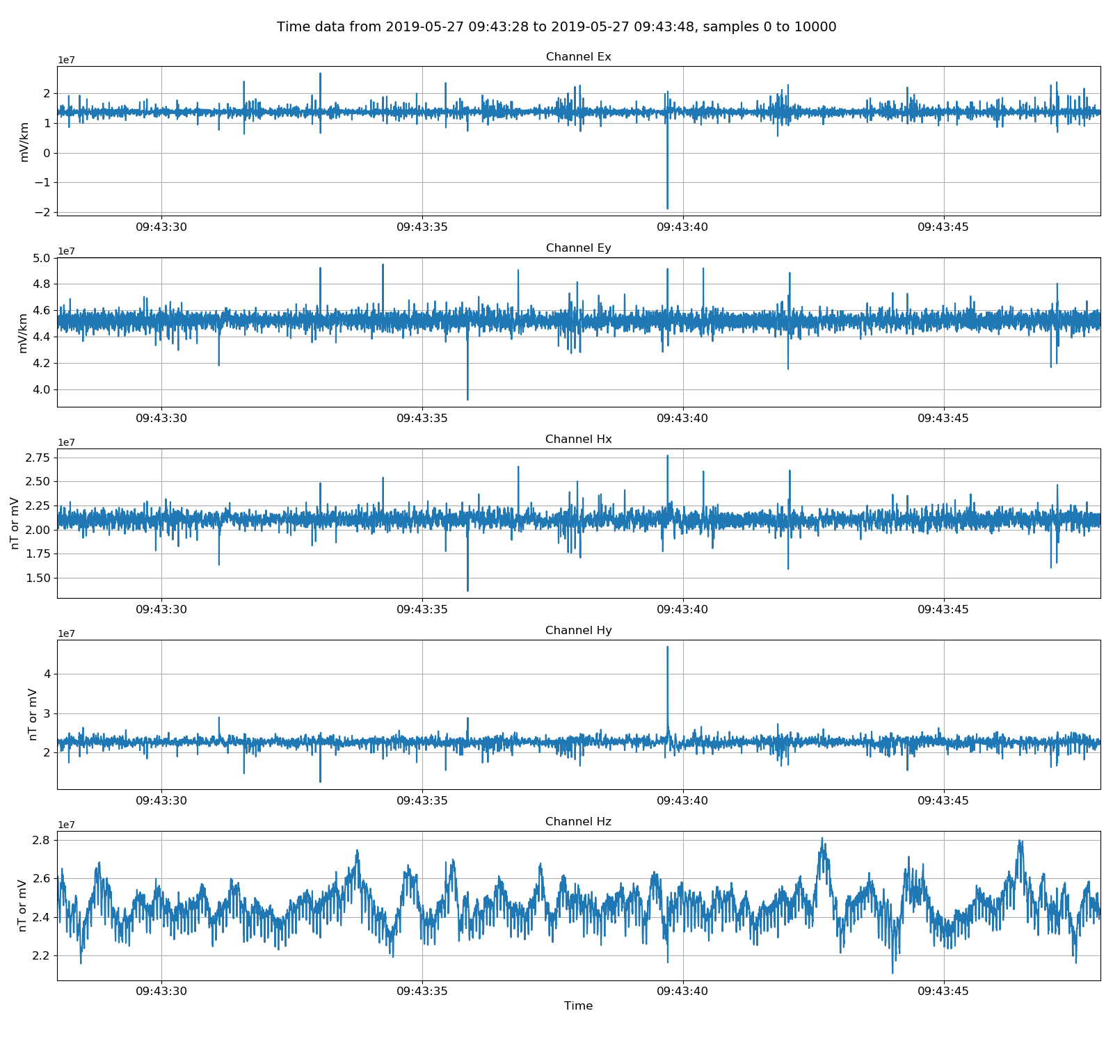
Viewing unscaled data. Units here are integer counts.
There are two stages of scaling in Lemi files:
The first converts the integer counts to microvolts for electric channels and mV for magnetic channels with the internal gain still applied. To get this data, the scale keyword to
getUnscaledSamples()needs to be set toTrue.The second scaling converts the microvolt electric channels to mV/km by also dividing by the diploe lengths in km. The gain on the magnetic channels is removed to give magnetic channels in mV. This is the resistics standard field units. The methods
getPhysicalSamples()orgetPhysicalData()will return aTimeDataobject in field units.
For example, to achieve scaling 1:
27 28 29 30 31 32 33 34 | startTime = "2019-05-27 15:00:00"
stopTime = "2019-05-27 15:00:15"
unscaledLemiData = lemiReader.getUnscaledData(startTime, stopTime, scale=True)
unscaledLemiData.printInfo()
fig = plt.figure(figsize=(16, 3 * unscaledLemiData.numChans))
unscaledLemiData.view(fig=fig, sampleStop=unscaledLemiData.numSamples)
fig.tight_layout(rect=[0, 0.02, 1, 0.96])
fig.savefig(timeImages / "lemiB423UnscaledWithScaleOption.png")
|
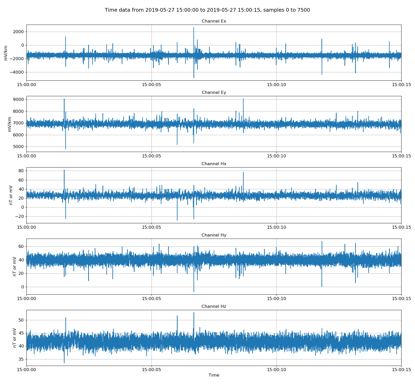
Viewing unscaled data. Units here are microvolts for electric channels and millivolts for magnetic channels with gain still applied.
Finally, to get data in field units of mV/km for electric channels and mV for magnetic channels, the methods getPhysicalSamples() or getPhysicalData() can be used like in the below example. This is equivalent to scaling situation 2 and returns the TimeData object in resistics standard field units.
36 37 38 39 40 41 | physicalLemiData = lemiReader.getPhysicalData(startTime, stopTime)
physicalLemiData.printInfo()
fig = plt.figure(figsize=(16, 3 * physicalLemiData.numChans))
physicalLemiData.view(fig=fig, sampleStop=physicalLemiData.numSamples)
fig.tight_layout(rect=[0, 0.02, 1, 0.96])
fig.savefig(timeImages / "lemiB423PhysicalData.png")
|
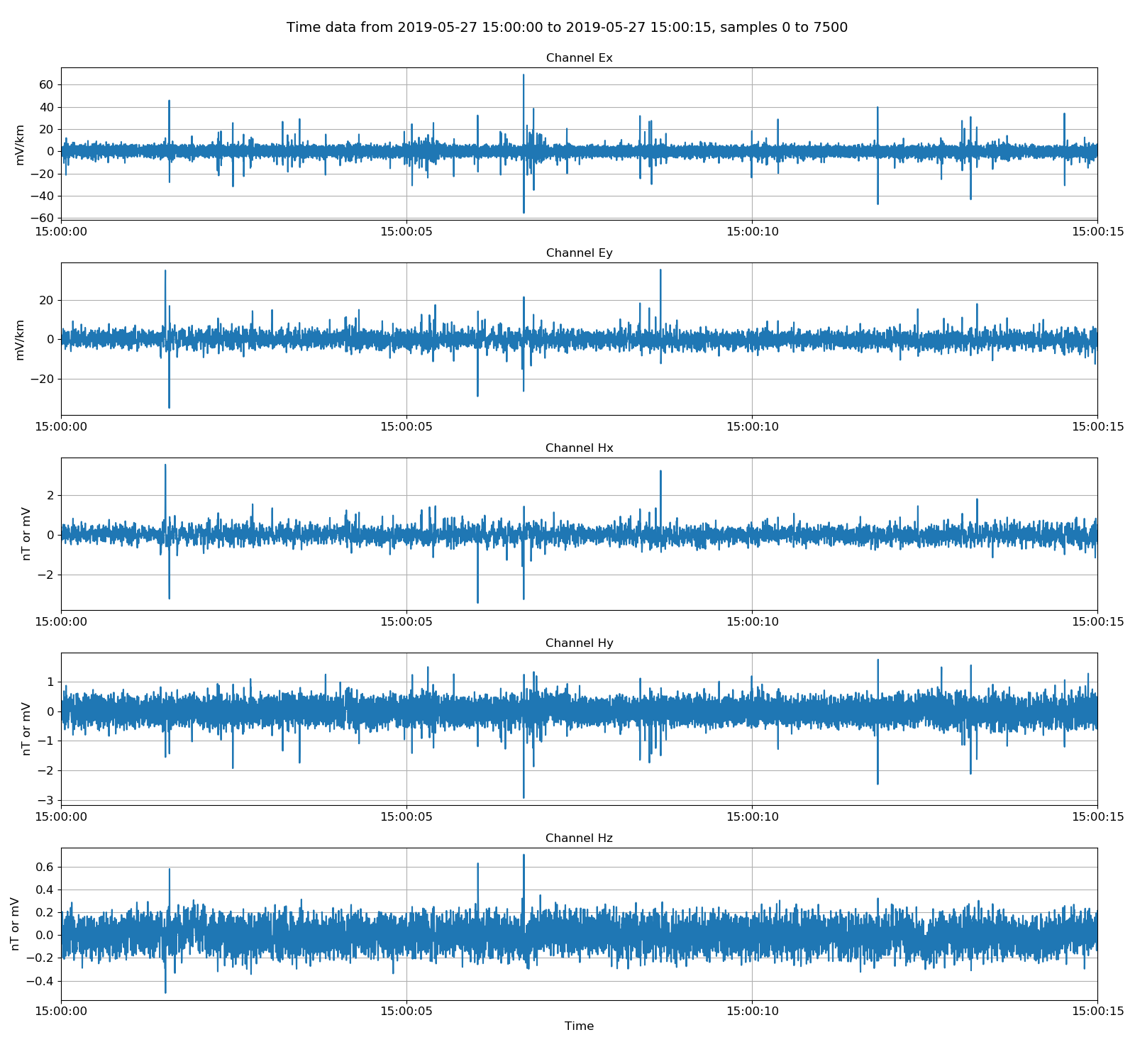
Viewing data in physical units. Electric channels in mV/km and magnetic channels in mV.
Much like the other data formats supported by resistics, Lemi B423 data can be written out in internal or ascii format.
43 44 45 46 47 48 49 | # write out as the internal format
from resistics.time.writer_internal import TimeWriterInternal
lemiB423_2internal = timePath / "lemiB423Internal"
writer = TimeWriterInternal()
writer.setOutPath(lemiB423_2internal)
writer.writeDataset(lemiReader, physical=True)
|
Reading in the internally formatted data, the dataset comments can be inspected.
51 52 53 54 55 | # read in the internal format dataset, see comments and plot original lemi data
from resistics.time.reader_internal import TimeReaderInternal
internalReader = TimeReaderInternal(lemiB423_2internal)
internalReader.printComments()
|
1 2 3 4 5 6 7 8 9 10 11 12 13 14 15 16 17 18 19 20 21 22 23 24 | Unscaled data 2019-05-27 09:43:28 to 2019-05-27 15:43:27 read in from measurement E:\magnetotellurics\code\resisticsdata\formats\timeData\lemiB423, samples 0 to 10799500
Sampling frequency 500.0
Data read from 2 files in total
Scaling = True
Scaling channel Hx of file E:\magnetotellurics\code\resisticsdata\formats\timeData\lemiB423\1558950203.B423 with multiplier 5.816314e-06 and adding -99.946
Scaling channel Hy of file E:\magnetotellurics\code\resisticsdata\formats\timeData\lemiB423\1558950203.B423 with multiplier 5.816975e-06 and adding -99.952
Scaling channel Hz of file E:\magnetotellurics\code\resisticsdata\formats\timeData\lemiB423\1558950203.B423 with multiplier 5.817061e-06 and adding -99.956
Scaling channel Ex of file E:\magnetotellurics\code\resisticsdata\formats\timeData\lemiB423\1558950203.B423 with multiplier 0.0002910952 and adding -5018.7
Scaling channel Ey of file E:\magnetotellurics\code\resisticsdata\formats\timeData\lemiB423\1558950203.B423 with multiplier 0.0002910181 and adding -4981.6
Scaling channel Hx of file E:\magnetotellurics\code\resisticsdata\formats\timeData\lemiB423\1558961007.B423 with multiplier 5.816314e-06 and adding -99.946
Scaling channel Hy of file E:\magnetotellurics\code\resisticsdata\formats\timeData\lemiB423\1558961007.B423 with multiplier 5.816975e-06 and adding -99.952
Scaling channel Hz of file E:\magnetotellurics\code\resisticsdata\formats\timeData\lemiB423\1558961007.B423 with multiplier 5.817061e-06 and adding -99.956
Scaling channel Ex of file E:\magnetotellurics\code\resisticsdata\formats\timeData\lemiB423\1558961007.B423 with multiplier 0.0002910952 and adding -5018.7
Scaling channel Ey of file E:\magnetotellurics\code\resisticsdata\formats\timeData\lemiB423\1558961007.B423 with multiplier 0.0002910181 and adding -4981.6
Removing gain of 16 from channel Hx
Removing gain of 16 from channel Hy
Removing gain of 16 from channel Hz
Dividing channel Ex by 1000 to convert microvolt to millivolt
Dividing channel Ex by electrode distance 0.06 km to give mV/km
Dividing channel Ey by 1000 to convert microvolt to millivolt
Dividing channel Ey by electrode distance 0.060700 km to give mV/km
Remove zeros: False, remove nans: False, remove average: True
Time series dataset written to E:\magnetotellurics\code\resisticsdata\formats\timeData\lemiB423Internal on 2019-10-05 18:13:59.133157 using resistics 0.0.6.dev2
---------------------------------------------------
|
The comment files in resistics detail the dataset history and the workflow to produce the dataset. They allow for easier reproducibility. For more information, see here.
The internally formatted data and the Lemi B423 data can be plotted together to make sure they are the same.
56 57 58 59 60 61 | physicalInternalData = internalReader.getPhysicalData(startTime, stopTime)
fig = plt.figure(figsize=(16, 3 * physicalLemiData.numChans))
physicalLemiData.view(fig=fig, sampleStop=500, label="Lemi B423 format")
physicalInternalData.view(fig=fig, sampleStop=500, label="Internal format", legend=True)
fig.tight_layout(rect=[0, 0.02, 1, 0.96])
fig.savefig(timeImages / "lemiB423_vs_internal.png")
|
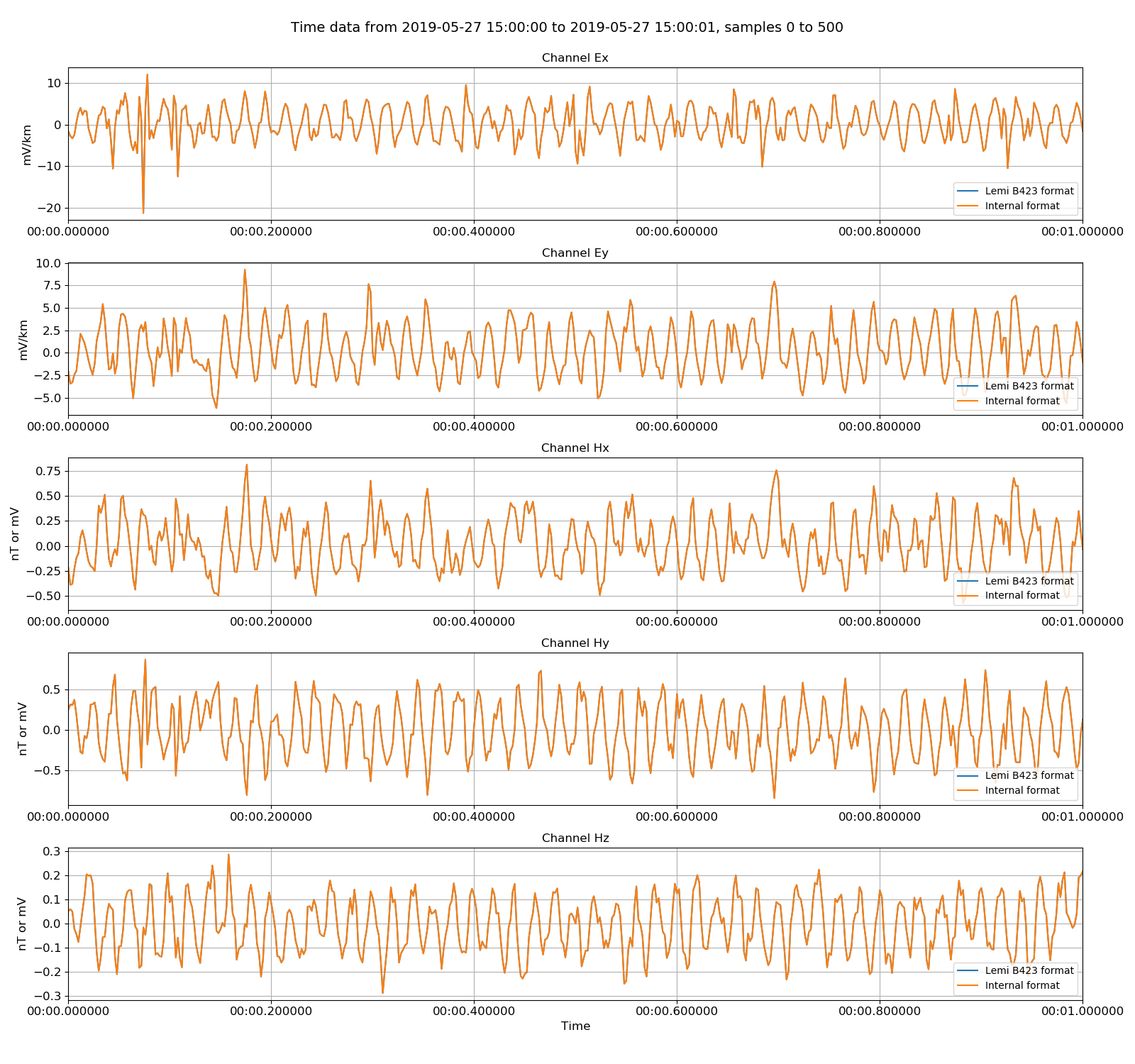
Lemi B423 data versus the internally formatted data. There are no differences.
Lemi B423E telluric headers
The Lemi B423E telluric format is similar to the Lemi B423 format. However, there are only four channels instead of five, namely, E1, E2, E3, E4. Again, headers need to be generated and for Lemi B423E, this is done using the measB423EHeaders() method of module reader_lemib423e. An example is shown below.
1 2 3 4 5 6 7 8 9 10 11 12 13 | from datapaths import timePath, timeImages
from resistics.time.reader_lemib423e import (
TimeReaderLemiB423E,
measB423EHeaders,
folderB423EHeaders,
)
lemiPath = timePath / "lemiB423E"
measB423EHeaders(lemiPath, 500, dx=60, dy=60.7, ex="E1", ey="E2")
lemiReader = TimeReaderLemiB423E(lemiPath)
lemiReader.printInfo()
lemiReader.printDataFileInfo()
|
To generate headers for a measurement, the following information needs to be provided:
The path to the folder with the Lemi B423E data files.
The sampling frequency in Hz of the data. In the above example, 500 Hz.
dx: the Ex dipole length
dy: the Ey dipole length
ex: The channel which is Ex. This is one of E1, E2, E3 or E4
ey: The channel which is Ey. This is one of E1, E2, E3 or E4
In this case, E1 maps to Ex and E2 maps to Ey. These channels will now be relabelled as Ex and Ey. Note that no electrodes were connected to either E3 or E4. The channel data for E3 and E4 is meaningless.
Before headers are generated, the measurement folder looks like this:
lemi01
├── 1558950203.B423
└── 1558961007.B423
And after, five header files with extension .h423E have been created. One global header and one header file each for channels E1, E2, E3 and E4.
lemi01
├── 1558950203.B423
├── 1558961007.B423
├── chan_00.h423E
├── chan_01.h423E
├── chan_02.h423E
├── chan_03.h423E
└── global.h423E
The global header file is included below.
1 2 3 4 5 6 7 8 | HEADER = GLOBAL
sample_freq = 500
num_samples = 10799501
start_time = 09:20:34.000000
start_date = 2019-05-27
stop_time = 15:20:33.000000
stop_date = 2019-05-27
meas_channels = 4
|
The channel header file for Ey is presented below. The channel header saves the information about the dipole length. The Ey dipole length is given by the absolute difference between pos_y2 and pos_y1.
1 2 3 4 5 6 7 8 9 10 11 12 13 14 15 16 17 18 19 20 21 22 23 | HEADER = CHANNEL
sample_freq = 500
num_samples = 10799501
start_time = 09:20:34.000000
start_date = 2019-05-27
stop_time = 15:20:33.000000
stop_date = 2019-05-27
ats_data_file = 1558948829.B423, 1558959633.B423
sensor_type =
channel_type = Ey
ts_lsb = 1
scaling_applied = False
pos_x1 = 0
pos_x2 = 1
pos_y1 = 0
pos_y2 = 60.7
pos_z1 = 0
pos_z2 = 1
sensor_sernum = 0
gain_stage1 = 1
gain_stage2 = 1
hchopper = 0
echopper = 0
|
The channel header file for E4 is shown below. As specified to the call to measB423EHeaders(), E1 and E2 have been mapped to Ex and Ey respectively. E3 and E4 are left unaltered and their dipole lengths remain as 1.
1 2 3 4 5 6 7 8 9 10 11 12 13 14 15 16 17 18 19 20 21 22 23 | HEADER = CHANNEL
sample_freq = 500
num_samples = 10799501
start_time = 09:20:34.000000
start_date = 2019-05-27
stop_time = 15:20:33.000000
stop_date = 2019-05-27
ats_data_file = 1558948829.B423, 1558959633.B423
sensor_type =
channel_type = E4
ts_lsb = 1
scaling_applied = False
pos_x1 = 0
pos_x2 = 1
pos_y1 = 0
pos_y2 = 1
pos_z1 = 0
pos_z2 = 1
sensor_sernum = 0
gain_stage1 = 1
gain_stage2 = 1
hchopper = 0
echopper = 0
|
Similarly to Lemi B423 data, header files can be created in a batch fashion for measurments in a folder where the parameters do not change. This is achieved using the folderB423EHeaders() method as shown below.
45 46 47 48 49 50 51 | # create headers for all measurements in a folder
folderPath = timePath / "lemiB423E_site"
folderB423EHeaders(folderPath, 500, dx=60, dy=60.7, ex="E1", ey="E2")
lemiPath = folderPath / "lemi01"
lemiReader = TimeReaderLemiB423E(lemiPath)
lemiReader.printInfo()
lemiReader.printDataFileInfo()
|
In this case, the folder structure before headers was:
lemiB423_site
├── lemi01
| └── 1558948829.B423
└── lemi01
└── 1558959633.B423
After generating the headers, the folder structure looks as below.
lemiB423_site
├── lemi01
| ├── 1558948829.B423
| ├── chan_00.h423
| ├── chan_01.h423
| ├── chan_02.h423
| ├── chan_03.h423
| ├── chan_04.h423
| └── global.h423
└── lemi01
├── 1558959633.B423
├── chan_00.h423
├── chan_01.h423
├── chan_02.h423
├── chan_03.h423
├── chan_04.h423
└── global.h423
Note
Once the header files are generated, the measurement data can be added to a resistics project and processed just as any other dataset.
Lemi B423E telluric data
Now the headers have been generated, the data can be read as normal. Similar to Lemi B423 data, the raw unscaled data is in integer counts and there are two sets of scaling that can be applied.
The first converts the integer counts to microvolts for electric channels. To get this data, the scale keyword to
getUnscaledSamples()needs to be set toTrue.The second scaling converts the microvolt electric channels to mV/km by also dividing by the diploe lengths in km. This is the resistics standard field units. The methods
getPhysicalSamples()orgetPhysicalData()will return aTimeDataobject in field units.
Plotting the integer counts can be achieved as follows:
15 16 17 18 19 20 21 22 23 24 25 | # plot data
import matplotlib.pyplot as plt
unscaledLemiData = lemiReader.getUnscaledSamples(
startSample=0, endSample=10000, scale=False
)
unscaledLemiData.printInfo()
fig = plt.figure(figsize=(16, 2 * unscaledLemiData.numChans))
unscaledLemiData.view(fig=fig, sampleStop=unscaledLemiData.numSamples)
fig.tight_layout(rect=[0, 0.02, 1, 0.96])
fig.savefig(timeImages / "lemiB423EUnscaled.png")
|
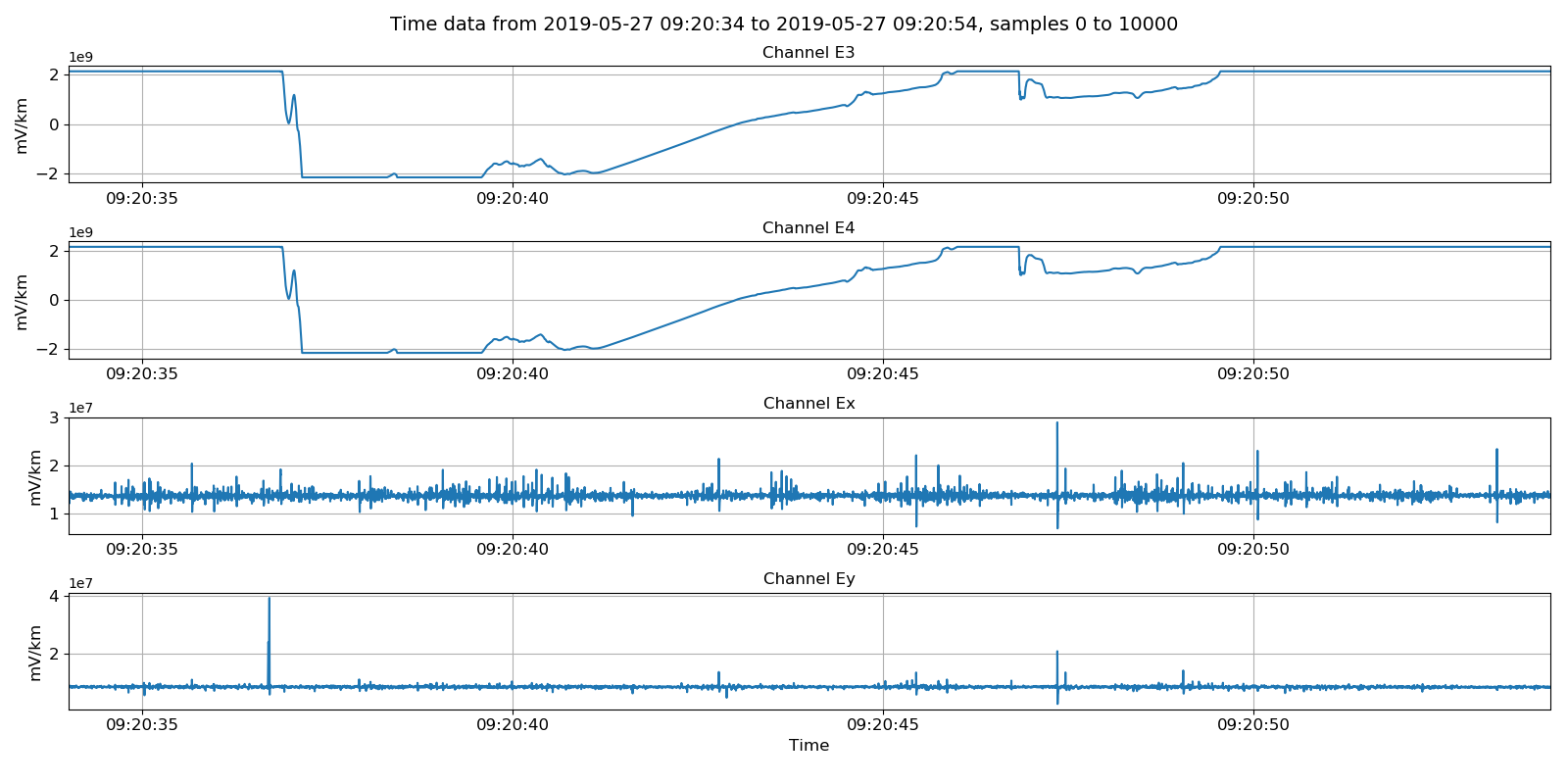
Viewing unscaled data. Units here are integer counts.
To get the electric channels in microvolts (and not corrected for dipole length):
27 28 29 30 31 32 33 34 | unscaledLemiData = lemiReader.getUnscaledSamples(
startSample=0, endSample=10000, scale=True
)
unscaledLemiData.printInfo()
fig = plt.figure(figsize=(16, 2 * unscaledLemiData.numChans))
unscaledLemiData.view(fig=fig, sampleStop=unscaledLemiData.numSamples)
fig.tight_layout(rect=[0, 0.02, 1, 0.96])
fig.savefig(timeImages / "lemiB423EUnscaledWithScaleOption.png")
|
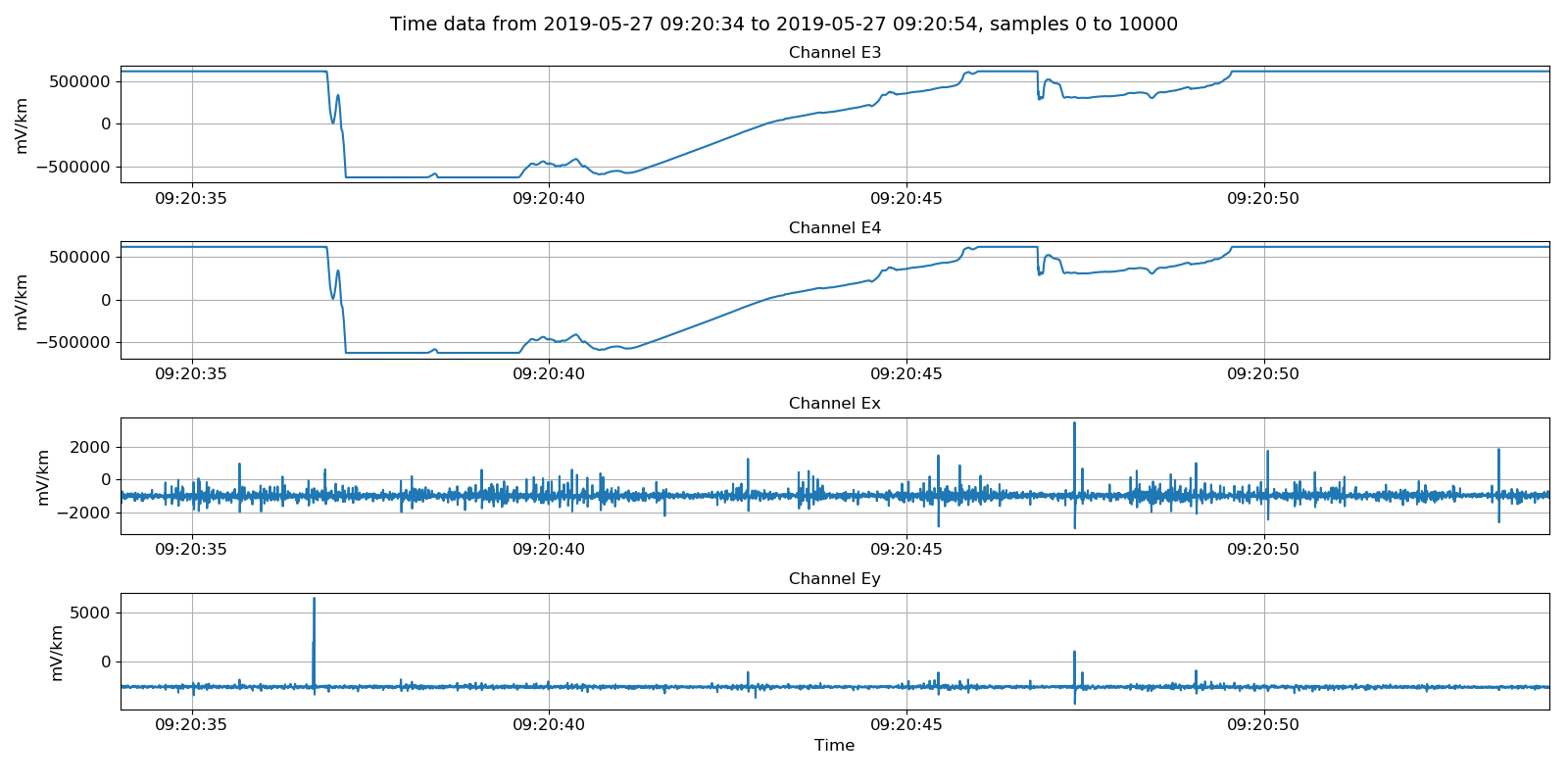
Viewing partially scaled units with electric channels in microvolts.
Finally, to get electric channels in field units, which is mV/km, the getPhysicalSamples() or getPhysicalData() methods can be used.
36 37 38 39 40 41 42 43 | physicalLemiData = lemiReader.getPhysicalSamples(
chans=["Ex", "Ey"], startSample=0, endSample=10000, remaverage=True
)
physicalLemiData.printInfo()
fig = plt.figure(figsize=(16, 3 * physicalLemiData.numChans))
physicalLemiData.view(fig=fig, sampleStop=physicalLemiData.numSamples)
fig.tight_layout(rect=[0, 0.02, 1, 0.96])
fig.savefig(timeImages / "lemiB423EPhysical.png")
|
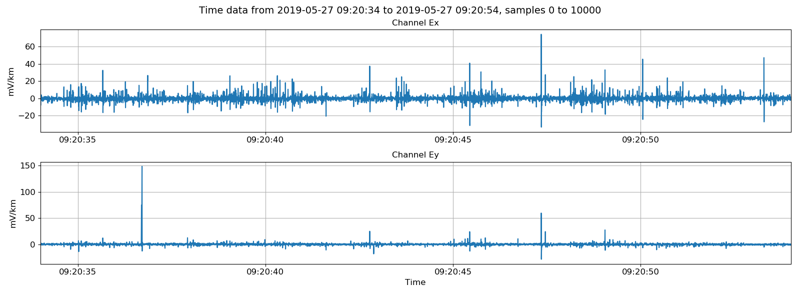
Viewing electric channels in mV/km or field units.
Complete example script
For the purposes of clarity, the complete example scripts are shown below.
For reading Lemi B423 magnetotelluric data.
1 2 3 4 5 6 7 8 9 10 11 12 13 14 15 16 17 18 19 20 21 22 23 24 25 26 27 28 29 30 31 32 33 34 35 36 37 38 39 40 41 42 43 44 45 46 47 48 49 50 51 52 53 54 55 56 57 58 59 60 61 62 63 64 65 66 67 68 69 70 71 72 | from datapaths import timePath, timeImages
from resistics.time.reader_lemib423 import (
TimeReaderLemiB423,
measB423Headers,
folderB423Headers,
)
lemiPath = timePath / "lemiB423"
measB423Headers(
lemiPath, 500, hxSensor=712, hySensor=710, hzSensor=714, hGain=16, dx=60, dy=60.7
)
lemiReader = TimeReaderLemiB423(lemiPath)
lemiReader.printInfo()
lemiReader.printDataFileInfo()
# plot data
import matplotlib.pyplot as plt
unscaledLemiData = lemiReader.getUnscaledSamples()
unscaledLemiData.printInfo()
fig = plt.figure(figsize=(16, 3 * unscaledLemiData.numChans))
unscaledLemiData.view(fig=fig, sampleStop=10000)
fig.tight_layout(rect=[0, 0.02, 1, 0.96])
fig.savefig(timeImages / "lemiB423Unscaled.png")
startTime = "2019-05-27 15:00:00"
stopTime = "2019-05-27 15:00:15"
unscaledLemiData = lemiReader.getUnscaledData(startTime, stopTime, scale=True)
unscaledLemiData.printInfo()
fig = plt.figure(figsize=(16, 3 * unscaledLemiData.numChans))
unscaledLemiData.view(fig=fig, sampleStop=unscaledLemiData.numSamples)
fig.tight_layout(rect=[0, 0.02, 1, 0.96])
fig.savefig(timeImages / "lemiB423UnscaledWithScaleOption.png")
physicalLemiData = lemiReader.getPhysicalData(startTime, stopTime)
physicalLemiData.printInfo()
fig = plt.figure(figsize=(16, 3 * physicalLemiData.numChans))
physicalLemiData.view(fig=fig, sampleStop=physicalLemiData.numSamples)
fig.tight_layout(rect=[0, 0.02, 1, 0.96])
fig.savefig(timeImages / "lemiB423PhysicalData.png")
# write out as the internal format
from resistics.time.writer_internal import TimeWriterInternal
lemiB423_2internal = timePath / "lemiB423Internal"
writer = TimeWriterInternal()
writer.setOutPath(lemiB423_2internal)
writer.writeDataset(lemiReader, physical=True)
# read in the internal format dataset, see comments and plot original lemi data
from resistics.time.reader_internal import TimeReaderInternal
internalReader = TimeReaderInternal(lemiB423_2internal)
internalReader.printComments()
physicalInternalData = internalReader.getPhysicalData(startTime, stopTime)
fig = plt.figure(figsize=(16, 3 * physicalLemiData.numChans))
physicalLemiData.view(fig=fig, sampleStop=500, label="Lemi B423 format")
physicalInternalData.view(fig=fig, sampleStop=500, label="Internal format", legend=True)
fig.tight_layout(rect=[0, 0.02, 1, 0.96])
fig.savefig(timeImages / "lemiB423_vs_internal.png")
# preparing headers for all measurement folders in a site
folderPath = timePath / "lemiB423_site"
folderB423Headers(
    folderPath, 500, hxSensor=712, hySensor=710, hzSensor=714, hGain=16, dx=60, dy=60.7
)

lemiPath = folderPath / "lemi01"
lemiReader = TimeReaderLemiB423(lemiPath)
lemiReader.printInfo()
lemiReader.printDataFileInfo()
|
And reading Lemi B423E telluric data.
1 2 3 4 5 6 7 8 9 10 11 12 13 14 15 16 17 18 19 20 21 22 23 24 25 26 27 28 29 30 31 32 33 34 35 36 37 38 39 40 41 42 43 44 45 46 47 48 49 50 51 | from datapaths import timePath, timeImages
from resistics.time.reader_lemib423e import (
TimeReaderLemiB423E,
measB423EHeaders,
folderB423EHeaders,
)
lemiPath = timePath / "lemiB423E"
measB423EHeaders(lemiPath, 500, dx=60, dy=60.7, ex="E1", ey="E2")
lemiReader = TimeReaderLemiB423E(lemiPath)
lemiReader.printInfo()
lemiReader.printDataFileInfo()
# plot data
import matplotlib.pyplot as plt
unscaledLemiData = lemiReader.getUnscaledSamples(
startSample=0, endSample=10000, scale=False
)
unscaledLemiData.printInfo()
fig = plt.figure(figsize=(16, 2 * unscaledLemiData.numChans))
unscaledLemiData.view(fig=fig, sampleStop=unscaledLemiData.numSamples)
fig.tight_layout(rect=[0, 0.02, 1, 0.96])
fig.savefig(timeImages / "lemiB423EUnscaled.png")
unscaledLemiData = lemiReader.getUnscaledSamples(
startSample=0, endSample=10000, scale=True
)
unscaledLemiData.printInfo()
fig = plt.figure(figsize=(16, 2 * unscaledLemiData.numChans))
unscaledLemiData.view(fig=fig, sampleStop=unscaledLemiData.numSamples)
fig.tight_layout(rect=[0, 0.02, 1, 0.96])
fig.savefig(timeImages / "lemiB423EUnscaledWithScaleOption.png")
physicalLemiData = lemiReader.getPhysicalSamples(
chans=["Ex", "Ey"], startSample=0, endSample=10000, remaverage=True
)
physicalLemiData.printInfo()
fig = plt.figure(figsize=(16, 3 * physicalLemiData.numChans))
physicalLemiData.view(fig=fig, sampleStop=physicalLemiData.numSamples)
fig.tight_layout(rect=[0, 0.02, 1, 0.96])
fig.savefig(timeImages / "lemiB423EPhysical.png")
# create headers for all measurements in a folder
folderPath = timePath / "lemiB423E_site"
folderB423EHeaders(folderPath, 500, dx=60, dy=60.7, ex="E1", ey="E2")
lemiPath = folderPath / "lemi01"
lemiReader = TimeReaderLemiB423E(lemiPath)
lemiReader.printInfo()
lemiReader.printDataFileInfo()
|