Internal binary format
A fair question to ask is why introduce another data format rather than use a pre-existing data format. The downsides of writing out in a pre-existing data format were the following:
Incorrect implementation
No control of specification
Makes the data no more portable
The internal format was chosen to achieve two main goals:
A binary format that allows easy portability
Headers written out in ascii that can be quickly checked
Therefore, numpy save was chosen as the method of writing the data. This means that the data is portable and can be opened by anyone with Python and the numpy package.
Internal format data folders tend to look like:
meas_2012-02-10_11-05-00
├── global.hdr
├── chan_00.hdr
├── chan_00.dat
├── chan_01.hdr
├── chan_01.dat
├── chan_02.hdr
├── chan_02.dat
├── chan_03.hdr
├── chan_03.dat
├── chan_04.hdr
├── chan_04.dat
└── comments.txt
The global header file contains the following information:
1 2 3 4 5 6 7 8 | HEADER = GLOBAL
sample_freq = 128.0
num_samples = 1783345
start_time = 02:35:00.000000
start_date = 2016-02-21
stop_time = 06:27:12.375000
stop_date = 2016-02-21
meas_channels = 5
|
And channel headers have channel specific header information:
1 2 3 4 5 6 7 8 9 10 11 12 13 14 15 16 17 18 19 20 21 22 23 | HEADER = CHANNEL
sample_freq = 128.0
num_samples = 1783345
start_time = 02:35:00.000000
start_date = 2016-02-21
stop_time = 06:27:12.375000
stop_date = 2016-02-21
ats_data_file = chan_00.dat
sensor_type = EFP06
channel_type = Ex
ts_lsb = -1.76666e-06
scaling_applied = True
pos_x1 = -45.0
pos_x2 = 41.0
pos_y1 = 0.0
pos_y2 = 0.0
pos_z1 = 0.0
pos_z2 = 0.0
sensor_sernum = 0
gain_stage1 = 16
gain_stage2 = 1
hchopper = 0
echopper = 0
|
Note
In order for resistics to recognise an internal formatted data folder, the following have to be present:
Header files with extension .hdr (global and one for each channel)
Data files with extension .dat
Note
In most cases, internally formatted data is written out from data already in field units. If the channel header scaling_applied is True, no scaling will be applied in either getUnscaledSamples() or getPhysicalSamples(). However, if scaling_applied is False, then getPhysicalSamples() will scale the data using the ts_lsb header and divide electric channels by the electrode spacing in km.
Internally formatted binary data is usually written out with comments in a separate file. An example comments file for internally formatted data is given below.
1 2 3 4 5 6 7 8 9 10 11 12 | Unscaled data 2016-02-21 02:35:00 to 2016-02-21 06:27:12.375000 read in from measurement E:\magnetotellurics\code\resisticsdata\formats\timeData\ats, samples 0 to 1783344
Sampling frequency 128.0
Scaling channel Ex with scalar -1.76666e-06 to give mV
Dividing channel Ex by electrode distance 0.086 km to give mV/km
Scaling channel Ey with scalar -1.76514e-06 to give mV
Dividing channel Ey by electrode distance 0.0861 km to give mV/km
Scaling channel Hx with scalar -0.000112802 to give mV
Scaling channel Hy with scalar -0.000225735 to give mV
Scaling channel Hz with scalar -1.41103e-05 to give mV
Remove zeros: False, remove nans: False, remove average: True
Time series dataset written to E:\magnetotellurics\code\resisticsdata\formats\timeData\atsInternal on 2019-10-05 18:09:07.436640 using resistics 0.0.6.dev2
---------------------------------------------------
|
The easiest method of formatting ASCII data as the internal binary format is to follow the instructions in the ASCII timeseries example.
The following will show how to read internally formatted binary data with numpy. To begin with, read an internally formatted dataset with the inbuilt TimeReaderInternal class.
1 2 3 4 5 6 7 | from datapaths import timePath, timeImages
from resistics.time.reader_internal import TimeReaderInternal
# data paths
internalPath = timePath / "atsInternal"
internalReader = TimeReaderInternal(internalPath)
internalReader.printInfo()
|
The printInfo() method shows information about the dataset, including various recording parameters.
1 2 3 4 5 6 7 8 9 10 11 12 13 14 15 16 17 18 19 20 21 22 23 24 25 26 | 13:17:35 DataReaderInternal: ####################
13:17:35 DataReaderInternal: DATAREADERINTERNAL INFO BEGIN
13:17:35 DataReaderInternal: ####################
13:17:35 DataReaderInternal: Data Path = timeData\atsInternal
13:17:35 DataReaderInternal: Global Headers
13:17:35 DataReaderInternal: {'sample_freq': 128.0, 'num_samples': 1783345, 'start_time': '02:35:00.000000', 'start_date': '2016-02-21', 'stop_time': '06:27:12.375000', 'stop_date': '2016-02-21', 'meas_channels': 5}
13:17:35 DataReaderInternal: Channels found:
13:17:35 DataReaderInternal: ['Ex', 'Ey', 'Hx', 'Hy', 'Hz']
13:17:35 DataReaderInternal: Channel Map
13:17:35 DataReaderInternal: {'Ex': 0, 'Ey': 1, 'Hx': 2, 'Hy': 3, 'Hz': 4}
13:17:35 DataReaderInternal: Channel Headers
13:17:35 DataReaderInternal: Ex
13:17:35 DataReaderInternal: {'sample_freq': 128.0, 'num_samples': 1783345, 'start_time': '02:35:00.000000', 'start_date': '2016-02-21', 'stop_time': '06:27:12.375000', 'stop_date': '2016-02-21', 'ats_data_file': 'chan_00.dat', 'sensor_type': 'EFP06', 'channel_type': 'Ex', 'ts_lsb': -1.76666e-06, 'scaling_applied': True, 'pos_x1': -45.0, 'pos_x2': 41.0, 'pos_y1': 0.0, 'pos_y2': 0.0, 'pos_z1': 0.0, 'pos_z2': 0.0, 'sensor_sernum': 0, 'gain_stage1': 16, 'gain_stage2': 1, 'hchopper': 0, 'echopper': 0}
13:17:35 DataReaderInternal: Ey
13:17:35 DataReaderInternal: {'sample_freq': 128.0, 'num_samples': 1783345, 'start_time': '02:35:00.000000', 'start_date': '2016-02-21', 'stop_time': '06:27:12.375000', 'stop_date': '2016-02-21', 'ats_data_file': 'chan_01.dat', 'sensor_type': 'EFP06', 'channel_type': 'Ey', 'ts_lsb': -1.76514e-06, 'scaling_applied': True, 'pos_x1': 0.0, 'pos_x2': 0.0, 'pos_y1': -45.0, 'pos_y2': 41.1, 'pos_z1': 0.0, 'pos_z2': 0.0, 'sensor_sernum': 0, 'gain_stage1': 16, 'gain_stage2': 1, 'hchopper': 0, 'echopper': 0}
13:17:35 DataReaderInternal: Hx
13:17:35 DataReaderInternal: {'sample_freq': 128.0, 'num_samples': 1783345, 'start_time': '02:35:00.000000', 'start_date': '2016-02-21', 'stop_time': '06:27:12.375000', 'stop_date': '2016-02-21', 'ats_data_file': 'chan_02.dat', 'sensor_type': 'MFS06e', 'channel_type': 'Hx', 'ts_lsb': -0.000112802, 'scaling_applied': True, 'pos_x1': 0.0, 'pos_x2': 0.0, 'pos_y1': 0.0, 'pos_y2': 0.0, 'pos_z1': 0.0, 'pos_z2': 0.0, 'sensor_sernum': 612, 'gain_stage1': 2, 'gain_stage2': 1, 'hchopper': 1, 'echopper': 0}
13:17:35 DataReaderInternal: Hy
13:17:35 DataReaderInternal: {'sample_freq': 128.0, 'num_samples': 1783345, 'start_time': '02:35:00.000000', 'start_date': '2016-02-21', 'stop_time': '06:27:12.375000', 'stop_date': '2016-02-21', 'ats_data_file': 'chan_03.dat', 'sensor_type': 'MFS06e', 'channel_type': 'Hy', 'ts_lsb': -0.000225735, 'scaling_applied': True, 'pos_x1': 0.0, 'pos_x2': 0.0, 'pos_y1': 0.0, 'pos_y2': 0.0, 'pos_z1': 0.0, 'pos_z2': 0.0, 'sensor_sernum': 613, 'gain_stage1': 1, 'gain_stage2': 1, 'hchopper': 1, 'echopper': 0}
13:17:35 DataReaderInternal: Hz
13:17:35 DataReaderInternal: {'sample_freq': 128.0, 'num_samples': 1783345, 'start_time': '02:35:00.000000', 'start_date': '2016-02-21', 'stop_time': '06:27:12.375000', 'stop_date': '2016-02-21', 'ats_data_file': 'chan_04.dat', 'sensor_type': 'MFS06e', 'channel_type': 'Hz', 'ts_lsb': -1.41103e-05, 'scaling_applied': True, 'pos_x1': 0.0, 'pos_x2': 0.0, 'pos_y1': 0.0, 'pos_y2': 0.0, 'pos_z1': 0.0, 'pos_z2': 0.0, 'sensor_sernum': 0, 'gain_stage1': 16, 'gain_stage2': 1, 'hchopper': 1, 'echopper': 0}
13:17:35 DataReaderInternal: Note: Field units used. Physical data has units mV/km for electric fields and mV for magnetic fields
13:17:35 DataReaderInternal: Note: To get magnetic field in nT, please calibrate
13:17:35 DataReaderInternal: ####################
13:17:35 DataReaderInternal: DATAREADERINTERNAL INFO END
13:17:35 DataReaderInternal: ####################
|
The TimeReaderInternal class does not automatically load the data into memory. Data has to be requested, which can be done using the getPhysicalSamples() or getUnscaledSamples() methods if all the data is required or only a sample range. To request data using dates, the getPhysicalData() or getUnscaledData() methods should be used. All of these return a TimeData object. In this case, a range of samples are requested and then information about the timeseries data is printed out to the terminal.
9 10 11 | # get data
internalData = internalReader.getPhysicalSamples(startSample=0, endSample=20000)
internalData.printInfo()
|
1 2 3 4 5 6 7 8 9 10 11 12 13 14 15 16 17 18 19 20 21 22 23 24 25 26 27 28 | 13:40:33 TimeData: ####################
13:40:33 TimeData: TIMEDATA INFO BEGIN
13:40:33 TimeData: ####################
13:40:33 TimeData: Sampling frequency [Hz] = 128.0
13:40:33 TimeData: Sample rate [s] = 0.0078125
13:40:33 TimeData: Number of samples = 20001
13:40:33 TimeData: Number of channels = 5
13:40:33 TimeData: Channels = ['Ex', 'Ey', 'Hx', 'Hy', 'Hz']
13:40:33 TimeData: Start time = 2016-02-21 02:35:00
13:40:33 TimeData: Stop time = 2016-02-21 02:37:36.250000
13:40:33 TimeData: Comments
13:40:33 TimeData: Unscaled data 2016-02-21 02:35:00 to 2016-02-21 06:27:12.375000 read in from measurement timeData\ats, samples 0 to 1783344
13:40:33 TimeData: Sampling frequency 128.0
13:40:33 TimeData: Scaling channel Ex with scalar -1.76666e-06 to give mV
13:40:33 TimeData: Dividing channel Ex by electrode distance 0.086 km to give mV/km
13:40:33 TimeData: Scaling channel Ey with scalar -1.76514e-06 to give mV
13:40:33 TimeData: Dividing channel Ey by electrode distance 0.0861 km to give mV/km
13:40:33 TimeData: Scaling channel Hx with scalar -0.000112802 to give mV
13:40:33 TimeData: Scaling channel Hy with scalar -0.000225735 to give mV
13:40:33 TimeData: Scaling channel Hz with scalar -1.41103e-05 to give mV
13:40:33 TimeData: Remove zeros: False, remove nans: False, remove average: True
13:40:33 TimeData: Dataset written to timeData\atsInternal on 2019-03-23 11:54:11.625577
13:40:33 TimeData: Unscaled data 2016-02-21 02:35:00 to 2016-02-21 02:37:36.250000 read in from measurement timeData\atsInternal, samples 0 to 20000
13:40:33 TimeData: Sampling frequency 128.0
13:40:33 TimeData: Remove zeros: False, remove nans: False, remove average: True
13:40:33 TimeData: ####################
13:40:33 TimeData: TIMEDATA INFO END
13:40:33 TimeData: ####################
|
The data can be plotted by using the view() method of TimeData. By passing a matplotlib figure, the layout of the plot can be further controlled.
13 14 15 16 17 18 19 20 | # plot
import matplotlib.pyplot as plt
fig = plt.figure(figsize=(16, 3 * internalData.numChans))
internalData.view(fig=fig, sampleStart=0, sampleStop=1000)
fig.tight_layout(rect=[0, 0.02, 1, 0.96])
plt.show()
fig.savefig(timeImages / "internalData.png")
|
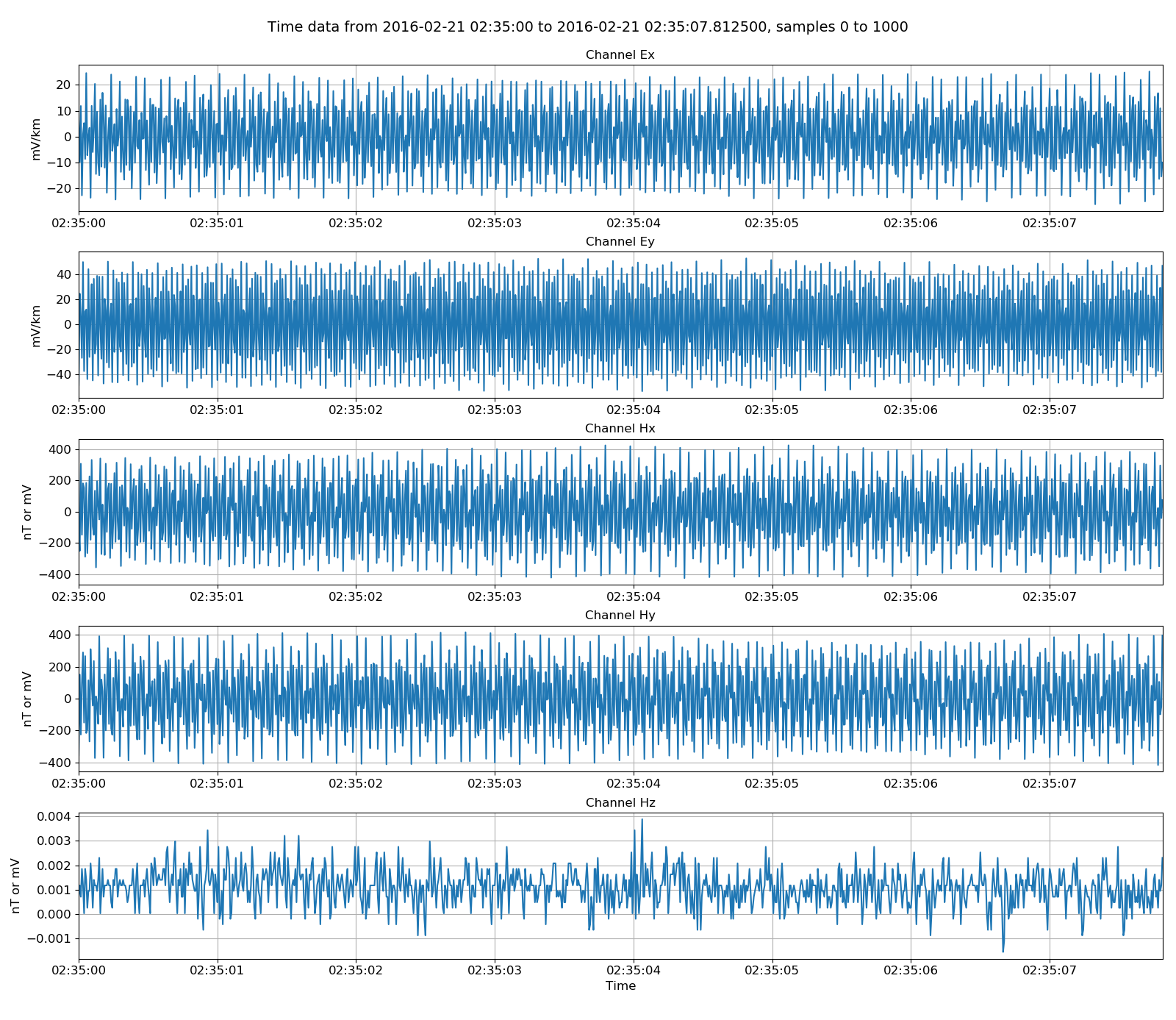
Viewing internal data
To show how the internal data format can be read using numpy, first create a map between channels and the channel data files. The map is simply a Python dictionary.
22 23 24 25 26 | # get the data file for each channel
channels = internalData.chans
chan2File = dict()
for chan in channels:
chan2File[chan] = internalReader.getChanDataFile(chan)
|
To read in channel Ex, all that is required is to use the numpy fromfile method and the filename along with a specification of the data type, which is np.float32 for data in field units.
28 29 30 31 32 | # read in the Ex data using numpy
import numpy as np
dataFile = internalPath / chan2File["Ex"]
npData = np.fromfile(str(dataFile), np.float32)
|
This method can be compared to the TimeReaderInternal class by plotting the two on the same plot. Matplotlib can help out with this.
34 35 36 37 38 39 40 | # plot the numpy data versus the internal format data
fig = plt.figure(figsize=(20, 4))
internalData.view(fig=fig, chans=["Ex"], sampleStart=0, sampleStop=250)
plt.plot(internalData.getDateArray()[0:251], npData[0:251], label="numpy read")
plt.legend()
fig.tight_layout(rect=[0, 0.02, 1, 0.96])
plt.show()
|
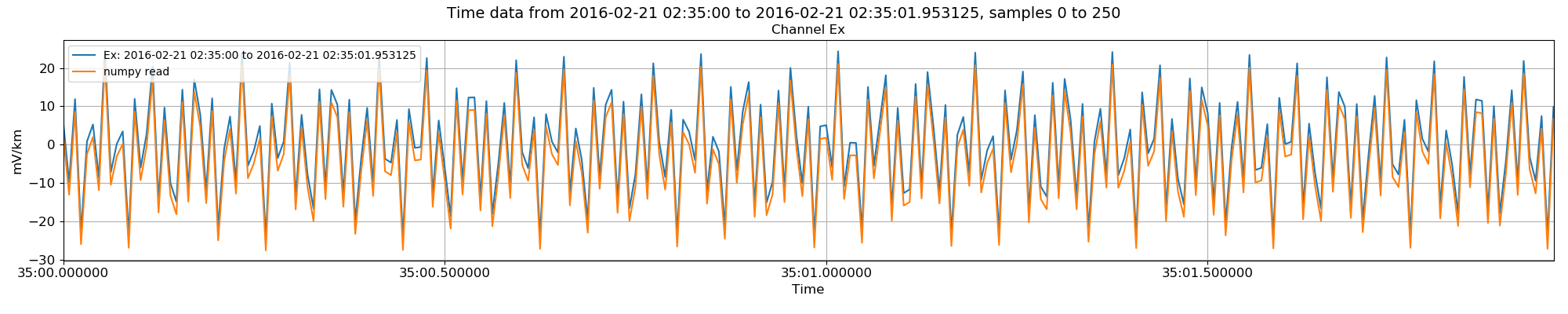
Internal data read in versus using numpy. There is a shift between the datasets.
As can be seen in the image, there is a shift between the two methods. This is because the get data methods of the various TimeReader classes return data minus the average value of the data. This can be optionally turned off as in the example below.
43 44 45 46 47 48 49 50 51 52 53 54 | # they do not look the same
# this is because of the average being removed in TimeReaderInternal.getPhysicalSamples()
# read the data again using TimeReaderInternal, but this time leave the average there
internalData = internalReader.getPhysicalSamples(
startSample=0, endSample=20000, remaverage=False
)
fig = plt.figure(figsize=(20, 4))
internalData.view(fig=fig, chans=["Ex"], sampleStart=0, sampleStop=250)
plt.plot(internalData.getDateArray()[0:251], npData[0:251], label="numpy read")
plt.legend(loc=2)
fig.tight_layout(rect=[0, 0.02, 1, 0.96])
plt.show()
|
Replotting the data now shows that the two are comparable.
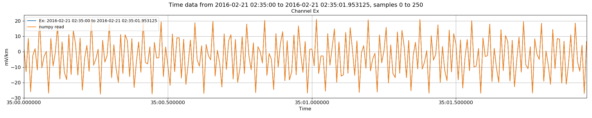
Internal data read (but without removing the average) in versus using numpy
Complete example script
For the purposes of clarity, the complete example script is shown below.
1 2 3 4 5 6 7 8 9 10 11 12 13 14 15 16 17 18 19 20 21 22 23 24 25 26 27 28 29 30 31 32 33 34 35 36 37 38 39 40 41 42 43 44 45 46 47 48 49 50 51 52 53 54 55 | from datapaths import timePath, timeImages
from resistics.time.reader_internal import TimeReaderInternal
# data paths
internalPath = timePath / "atsInternal"
internalReader = TimeReaderInternal(internalPath)
internalReader.printInfo()
# get data
internalData = internalReader.getPhysicalSamples(startSample=0, endSample=20000)
internalData.printInfo()
# plot
import matplotlib.pyplot as plt

fig = plt.figure(figsize=(16, 3 * internalData.numChans))
internalData.view(fig=fig, sampleStart=0, sampleStop=1000)
fig.tight_layout(rect=[0, 0.02, 1, 0.96])
plt.show()
fig.savefig(timeImages / "internalData.png")
# get the data file for each channel
channels = internalData.chans
chan2File = dict()
for chan in channels:
    chan2File[chan] = internalReader.getChanDataFile(chan)
# read in the Ex data using numpy
import numpy as np

dataFile = internalPath / chan2File["Ex"]
npData = np.fromfile(str(dataFile), np.float32)
# plot the numpy data versus the internal format data
fig = plt.figure(figsize=(20, 4))
internalData.view(fig=fig, chans=["Ex"], sampleStart=0, sampleStop=250)
plt.plot(internalData.getDateArray()[0:251], npData[0:251], label="numpy read")
plt.legend()
fig.tight_layout(rect=[0, 0.02, 1, 0.96])
plt.show()
fig.savefig(timeImages / "internalData_vs_npLoad.png")
# they do not look the same
# this is because of the average being removed in TimeReaderInternal.getPhysicalSamples()
# read the data again using TimeReaderInternal, but this time leave the average there
internalData = internalReader.getPhysicalSamples(
    startSample=0, endSample=20000, remaverage=False
)
fig = plt.figure(figsize=(20, 4))
internalData.view(fig=fig, chans=["Ex"], sampleStart=0, sampleStop=250)
plt.plot(internalData.getDateArray()[0:251], npData[0:251], label="numpy read")
plt.legend(loc=2)
fig.tight_layout(rect=[0, 0.02, 1, 0.96])
plt.show()
fig.savefig(timeImages / "internalDataWithAvg_vs_npLoad.png")
|