Phoenix timeseries
Phoenix recordings are the most challenging to support as they do not nicely fit the resistics model of data. A typical phoenix data directory will have a .tbl header file and three data files, one for three different sampling frequencies.
phnx01
├── 1463N13.TBL
├── 1463N13.TS3
├── 1463N13.TS4
└── 1463N13.TS5
The highest TS number is the file with the continuously sampled data, which is normally the lowest sampling frequency.
Note
In order for resistics to recognise a Phoenix data folder, the following have to be present:
A header file with extension .TBL
Data files with extension .TS? where ? represents an integer
Warning
The scaling currently applied for phoenix data has not been verified and requires further testing. Therefore, it is not currently known how to calibrate the data.
Phoenix binary formatted calibration files are also not supported but ASCII files can be used instead as required.
Phoenix recordings are opened in resistics using the TimeReaderPhoenix class. An example is provided below:
1 2 3 4 5 6 7 8 | from datapaths import timePath, timeImages
from resistics.time.reader_phoenix import TimeReaderPhoenix
# read in spam data
phoenixPath = timePath / "phoenix"
phoenixReader = TimeReaderPhoenix(phoenixPath)
phoenixReader.printDataFileInfo()
phoenixReader.printInfo()
|
The phoenix data reader can show information about the sampling frequencies for the various data files by using the printDataFileList() method.
1 2 3 4 5 6 7 8 9 10 11 | 16:49:46 DataReaderPhoenix Data File List: ####################
16:49:46 DataReaderPhoenix Data File List: DATAREADERPHOENIX DATA FILE LIST INFO BEGIN
16:49:46 DataReaderPhoenix Data File List: ####################
16:49:46 DataReaderPhoenix Data File List: TS File Sampling frequency (Hz) Num Samples
16:49:46 DataReaderPhoenix Data File List: 1463N13.TS3 2400 3086400
16:49:46 DataReaderPhoenix Data File List: 1463N13.TS4 150 1542750
16:49:46 DataReaderPhoenix Data File List: 1463N13.TS5 15 1157175
16:49:46 DataReaderPhoenix Data File List: Continuous data file: 1463N13.TS5
16:49:46 DataReaderPhoenix Data File List: ####################
16:49:46 DataReaderPhoenix Data File List: DATAREADERPHOENIX DATA FILE LIST INFO END
16:49:46 DataReaderPhoenix Data File List: ####################
|
Three data files are listed, along with their sampling frequencies and the number of samples in each. Further, the continuous recording file is shown.
The phoenix data reader essentially only supports the continuous data file. When data is requested, only data from the continuous data channel is returned. Similarly, headers refer to the continuous recording data file as can been seen when printing the recording information out using phoenixReader.printInfo().
1 2 3 4 5 6 7 8 9 10 11 12 13 14 15 16 17 18 19 20 21 22 23 24 25 26 | 16:28:20 DataReaderPhoenix: ####################
16:28:20 DataReaderPhoenix: DATAREADERPHOENIX INFO BEGIN
16:28:20 DataReaderPhoenix: ####################
16:28:20 DataReaderPhoenix: Data Path = timeData\phoenix
16:28:20 DataReaderPhoenix: Global Headers
16:28:20 DataReaderPhoenix: {'sample_freq': 15.0, 'start_date': '2011-11-13', 'start_time': '17:04:02.000', 'stop_date': '2011-11-14', 'stop_time': '14:29:46.933333', 'num_samples': 1157175, 'ats_data_file': 'timeData\\phoenix\\1463N13.TS5', 'meas_channels': 5}
16:28:20 DataReaderPhoenix: Channels found:
16:28:20 DataReaderPhoenix: ['Ex', 'Ey', 'Hx', 'Hy', 'Hz']
16:28:20 DataReaderPhoenix: Channel Map
16:28:20 DataReaderPhoenix: {'Ex': 0, 'Ey': 1, 'Hx': 2, 'Hy': 3, 'Hz': 4}
16:28:20 DataReaderPhoenix: Channel Headers
16:28:20 DataReaderPhoenix: Ex
16:28:20 DataReaderPhoenix: {'gain_stage1': 10, 'gain_stage2': 1, 'hchopper': 0, 'echopper': 0, 'ats_data_file': 'timeData\\phoenix\\1463N13.TS5', 'num_samples': 1157175, 'sensor_type': '', 'channel_type': 'Ex', 'ts_lsb': 1.0, 'scaling_applied': False, 'pos_x1': 46.5, 'pos_x2': 46.5, 'pos_y1': 0.0, 'pos_y2': 0.0, 'pos_z1': 0.0, 'pos_z2': 0.0, 'sensor_sernum': 0, 'sample_freq': 15.0}
16:28:20 DataReaderPhoenix: Ey
16:28:20 DataReaderPhoenix: {'gain_stage1': 10, 'gain_stage2': 1, 'hchopper': 0, 'echopper': 0, 'ats_data_file': 'timeData\\phoenix\\1463N13.TS5', 'num_samples': 1157175, 'sensor_type': '', 'channel_type': 'Ey', 'ts_lsb': 1.0, 'scaling_applied': False, 'pos_x1': 0.0, 'pos_x2': 0.0, 'pos_y1': 46.5, 'pos_y2': 46.5, 'pos_z1': 0.0, 'pos_z2': 0.0, 'sensor_sernum': 0, 'sample_freq': 15.0}
16:28:20 DataReaderPhoenix: Hx
16:28:20 DataReaderPhoenix: {'gain_stage1': 12, 'gain_stage2': 1, 'hchopper': 0, 'echopper': 0, 'ats_data_file': 'timeData\\phoenix\\1463N13.TS5', 'num_samples': 1157175, 'sensor_type': 'Phoenix', 'channel_type': 'Hx', 'ts_lsb': 1.0, 'scaling_applied': False, 'pos_x1': 0.0, 'pos_x2': 0.0, 'pos_y1': 0.0, 'pos_y2': 0.0, 'pos_z1': 0.0, 'pos_z2': 0.0, 'sensor_sernum': 1424, 'sample_freq': 15.0}
16:28:20 DataReaderPhoenix: Hy
16:28:20 DataReaderPhoenix: {'gain_stage1': 12, 'gain_stage2': 1, 'hchopper': 0, 'echopper': 0, 'ats_data_file': 'timeData\\phoenix\\1463N13.TS5', 'num_samples': 1157175, 'sensor_type': 'Phoenix', 'channel_type': 'Hy', 'ts_lsb': 1.0, 'scaling_applied': False, 'pos_x1': 0.0, 'pos_x2': 0.0, 'pos_y1': 0.0, 'pos_y2': 0.0, 'pos_z1': 0.0, 'pos_z2': 0.0, 'sensor_sernum': 1425, 'sample_freq': 15.0}
16:28:20 DataReaderPhoenix: Hz
16:28:20 DataReaderPhoenix: {'gain_stage1': 12, 'gain_stage2': 1, 'hchopper': 0, 'echopper': 0, 'ats_data_file': 'timeData\\phoenix\\1463N13.TS5', 'num_samples': 1157175, 'sensor_type': 'Phoenix', 'channel_type': 'Hz', 'ts_lsb': 1.0, 'scaling_applied': False, 'pos_x1': 0.0, 'pos_x2': 0.0, 'pos_y1': 0.0, 'pos_y2': 0.0, 'pos_z1': 0.0, 'pos_z2': 0.0, 'sensor_sernum': 1426, 'sample_freq': 15.0}
16:28:20 DataReaderPhoenix: Note: Field units used. Physical data has units mV/km for electric fields and mV for magnetic fields
16:28:20 DataReaderPhoenix: Note: To get magnetic field in nT, please calibrate
16:28:20 DataReaderPhoenix: ####################
16:28:20 DataReaderPhoenix: DATAREADERPHOENIX INFO END
16:28:20 DataReaderPhoenix: ####################
|
Much like the other data readers, there are both global headers, which apply to all the channels, and channel specific headers.
Resistics does not immediately load timeseries data into memory. In order to read the data from the files, it needs to be requested.
10 11 12 13 14 | # get some data
startTime = "2011-11-14 02:00:00"
stopTime = "2011-11-14 03:00:00"
unscaledData = phoenixReader.getUnscaledData(startTime, stopTime)
print(unscaledData)
|
phoenixReader.getUnscaledData(startTime, stopTime) will read timeseries data from the data files and returns a TimeData object with data in the raw data units. Alternatively, to get all the data without any time restrictions, use phoenixReader.getUnscaledSamples().
Information about the time data can be printed using either unscaledData.printInfo() or simply print(unscaledData). An example of the time data information is below:
1 2 3 4 5 6 7 8 9 10 11 12 13 14 15 | 16:49:46 TimeData: ####################
16:49:46 TimeData: TIMEDATA INFO BEGIN
16:49:46 TimeData: ####################
16:49:46 TimeData: Sampling frequency [Hz] = 15.0
16:49:46 TimeData: Sample rate [s] = 0.06666666666666667
16:49:46 TimeData: Number of samples = 54001
16:49:46 TimeData: Number of channels = 5
16:49:46 TimeData: Channels = ['Ex', 'Ey', 'Hx', 'Hy', 'Hz']
16:49:46 TimeData: Start time = 2011-11-14 02:00:00
16:49:46 TimeData: Stop time = 2011-11-14 03:00:00
16:49:46 TimeData: Comments
16:49:46 TimeData: Unscaled data 2011-11-14 02:00:00 to 2011-11-14 03:00:00 read in from measurement timeData\phoenix, samples 482370 to 536370
16:49:46 TimeData: ####################
16:49:46 TimeData: TIMEDATA INFO END
16:49:46 TimeData: ####################
|
After reading in some data, it is natural to view it. Time data can be viewed using the view() method of the class. By additionally providing a matplotlib figure object, the style and layout of the plot can be controlled.
16 17 18 19 20 21 22 23 | # plot data
import matplotlib.pyplot as plt
fig = plt.figure(figsize=(16, 3 * unscaledData.numChans))
unscaledData.view(fig=fig, sampleEnd=20000)
fig.tight_layout(rect=[0, 0.02, 1, 0.96])
plt.show()
fig.savefig(timeImages / "phoenixUnscaled.png")
|
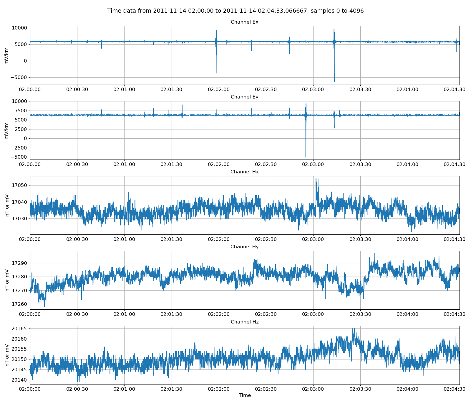
Viewing unscaled data
Unscaled data is generally not of use. More useful is data scaled to physically meaningful units. Resistics uses magnetotelluric field units and the method,
phoenixReader.getPhysicalData(startTime, stopTime)
returns a time data object in physical units. This time data object can also be visualised.
25 26 27 28 29 30 31 32 | # let's try physical data and view it
physicalData = phoenixReader.getPhysicalData(startTime, stopTime)
physicalData.printInfo()
fig = plt.figure(figsize=(16, 3 * physicalData.numChans))
physicalData.view(fig=fig, sampleEnd=20000)
fig.tight_layout(rect=[0, 0.02, 1, 0.96])
plt.show()
fig.savefig(timeImages / "phoenixPhysical.png")
|
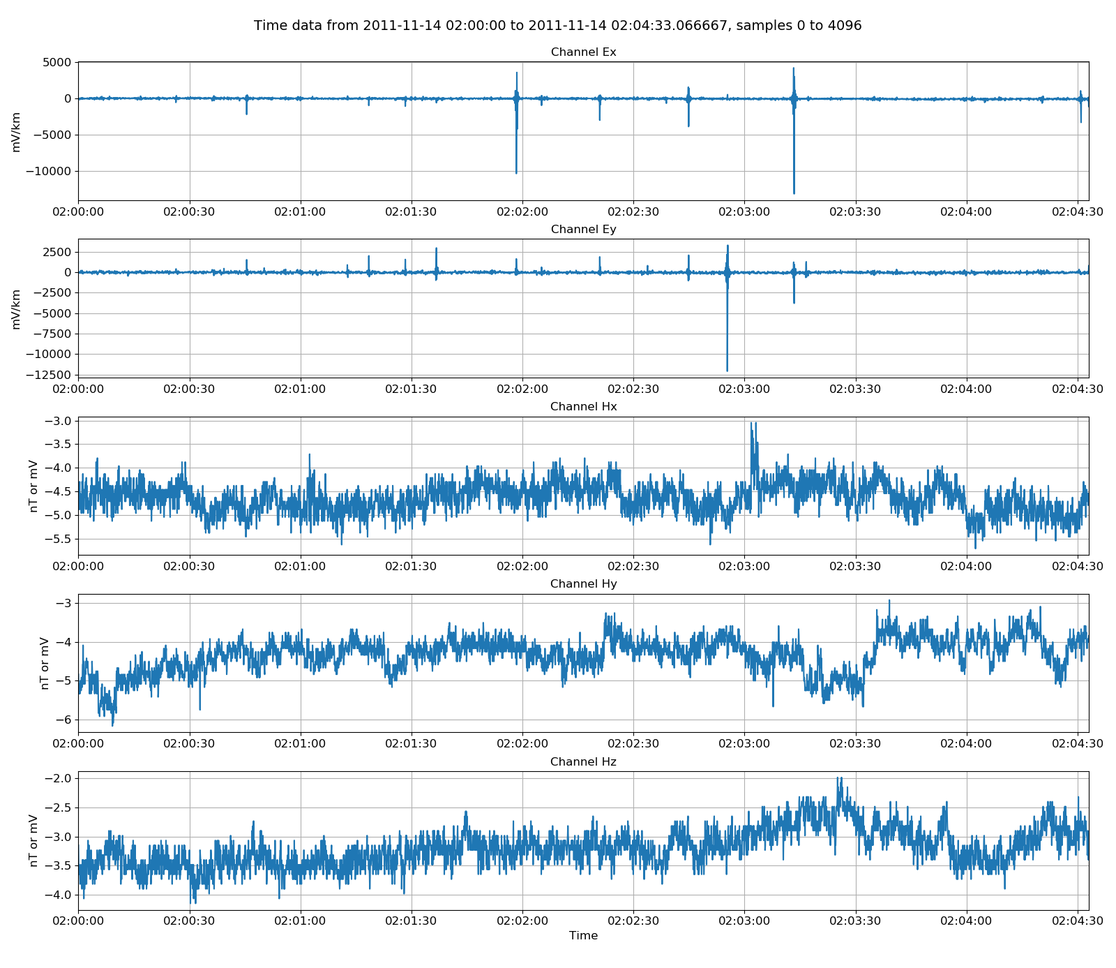
Viewing physically scaled data
There are a few helpful methods built in to resistics for manipulating time series data. These are generally in filter. In the example below, the time data is high pass filtered 4 Hz and then plotted.
34 35 36 37 38 39 40 41 42 | # can filter the data
from resistics.time.filter import highPass
filteredData = highPass(physicalData, 4, inplace=False)
fig = plt.figure(figsize=(16, 3 * physicalData.numChans))
filteredData.view(fig=fig, sampleEnd=20000)
fig.tight_layout(rect=[0, 0.02, 1, 0.96])
plt.show()
fig.savefig(timeImages / "phoenixFiltered.png")
|
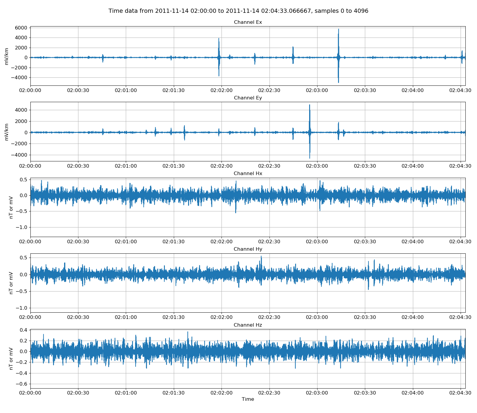
Viewing physically scaled and then high pass filtered data
The phoenix reader has a helpful function for reformatting the continuous phoenix channel to the internal binary data format. The below example shows how this is done:
44 45 46 | # reformat the continuous sampling frequency
phoenix_2internal = timePath / "phoenixInternal"
phoenixReader.reformatContinuous(phoenix_2internal)
|
To check the fidelity of this function, the internally formatted data can be read back in and plotted with the original data. To read the data back in, use the TimeReaderInternal class.
48 49 50 51 52 53 54 55 | # reading output
from resistics.time.reader_internal import TimeReaderInternal
internalReader = TimeReaderInternal(
phoenix_2internal / "meas_ts5_2011-11-13-17-04-02_2011-11-14-14-29-46"
)
internalReader.printInfo()
internalReader.printComments()
|
The comments of this reformatted dataset show the various scalings and modifications that have been applied to the data.
1 2 3 4 5 6 7 8 9 10 11 12 | Unscaled data 2011-11-13 17:04:02 to 2011-11-14 14:29:46.933333 read in from measurement E:\magnetotellurics\code\resisticsdata\formats\timeData\phoenix, samples 0 to 1157174
Scaling channel Ex with scalar 0.1 to give mV
Dividing channel Ex by electrode distance 0.093 km to give mV/km
Scaling channel Ey with scalar 0.1 to give mV
Dividing channel Ey by electrode distance 0.093 km to give mV/km
Scaling channel Hx with scalar 0.08333333333333333 to give mV
Scaling channel Hy with scalar 0.08333333333333333 to give mV
Scaling channel Hz with scalar 0.08333333333333333 to give mV
The required Phoneix scaling to field units is still unverified. This is experimental and use cautiously.
Remove zeros: False, remove nans: False, remove average: True
Time series dataset written to E:\magnetotellurics\code\resisticsdata\formats\timeData\phoenixInternal\meas_ts5_2011-11-13-17-04-02_2011-11-14-14-29-46 on 2019-10-05 18:14:54.116435 using resistics 0.0.6.dev2
---------------------------------------------------
|
The datasets can be compared by plotting them together. First, read in some physical data from the internal time data reader.
57 58 | # read in physical data
internalData = internalReader.getPhysicalData(startTime, stopTime)
|
And then plot both the original data and the internally formatted data on the same plot:
60 61 62 63 64 65 66 | # plot the two together
fig = plt.figure(figsize=(16, 3 * physicalData.numChans))
physicalData.view(fig=fig, label="Phoenix format data")
internalData.view(fig=fig, label="Internal format data", legend=True)
fig.tight_layout(rect=[0, 0.02, 1, 0.96])
plt.show()
fig.savefig(timeImages / "phoenix_vs_internal_continuous.png")
|
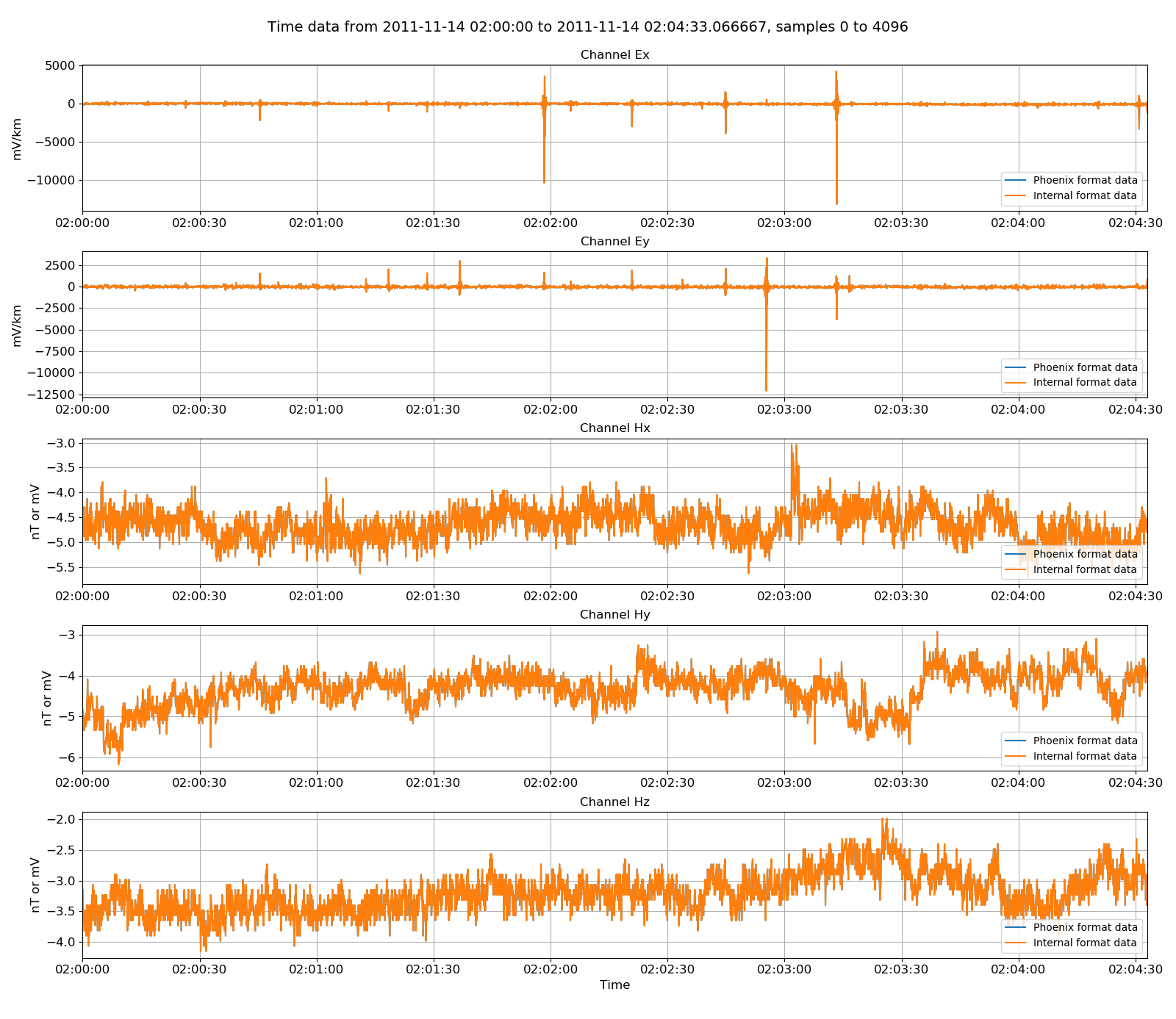
Phoenix original data versus the reformatted data in the internal data format
Complete example script
For the purposes of clarity, the complete example script is shown below.
1 2 3 4 5 6 7 8 9 10 11 12 13 14 15 16 17 18 19 20 21 22 23 24 25 26 27 28 29 30 31 32 33 34 35 36 37 38 39 40 41 42 43 44 45 46 47 48 49 50 51 52 53 54 55 56 57 58 59 60 61 62 63 64 65 66 | from datapaths import timePath, timeImages
from resistics.time.reader_phoenix import TimeReaderPhoenix
# read in spam data
phoenixPath = timePath / "phoenix"
phoenixReader = TimeReaderPhoenix(phoenixPath)
phoenixReader.printDataFileInfo()
phoenixReader.printInfo()
# get some data
startTime = "2011-11-14 02:00:00"
stopTime = "2011-11-14 03:00:00"
unscaledData = phoenixReader.getUnscaledData(startTime, stopTime)
print(unscaledData)
# plot data
import matplotlib.pyplot as plt

fig = plt.figure(figsize=(16, 3 * unscaledData.numChans))
unscaledData.view(fig=fig, sampleEnd=20000)
fig.tight_layout(rect=[0, 0.02, 1, 0.96])
plt.show()
fig.savefig(timeImages / "phoenixUnscaled.png")
# let's try physical data and view it
physicalData = phoenixReader.getPhysicalData(startTime, stopTime)
physicalData.printInfo()
fig = plt.figure(figsize=(16, 3 * physicalData.numChans))
physicalData.view(fig=fig, sampleEnd=20000)
fig.tight_layout(rect=[0, 0.02, 1, 0.96])
plt.show()
fig.savefig(timeImages / "phoenixPhysical.png")
# can filter the data
from resistics.time.filter import highPass

filteredData = highPass(physicalData, 4, inplace=False)
fig = plt.figure(figsize=(16, 3 * physicalData.numChans))
filteredData.view(fig=fig, sampleEnd=20000)
fig.tight_layout(rect=[0, 0.02, 1, 0.96])
plt.show()
fig.savefig(timeImages / "phoenixFiltered.png")
# reformat the continuous sampling frequency
phoenix_2internal = timePath / "phoenixInternal"
phoenixReader.reformatContinuous(phoenix_2internal)
# reading output
from resistics.time.reader_internal import TimeReaderInternal

internalReader = TimeReaderInternal(
    phoenix_2internal / "meas_ts5_2011-11-13-17-04-02_2011-11-14-14-29-46"
)
internalReader.printInfo()
internalReader.printComments()
# read in physical data
internalData = internalReader.getPhysicalData(startTime, stopTime)
# plot the two together
fig = plt.figure(figsize=(16, 3 * physicalData.numChans))
physicalData.view(fig=fig, label="Phoenix format data")
internalData.view(fig=fig, label="Internal format data", legend=True)
fig.tight_layout(rect=[0, 0.02, 1, 0.96])
plt.show()
fig.savefig(timeImages / "phoenix_vs_internal_continuous.png")
|