Interpolation to second
For best results, resistics requires data to be sampled on the second. For an example of a dataset not sampled on the second, consider recording at 10 Hz, with the first sample at 0.05 seconds. Then the sample times will be:
0.05 0.15 0.25 0.35 0.45 0.55 0.65 0.75 0.85 0.95 1.05 1.15 1.25 ...
Interpolating to the second will change the sample times to:
0.10 0.20 0.30 0.40 0.50 0.60 0.70 0.80 0.90 1.00 1.10 1.20 ...
The easiest way to show how to do this is with a practical example. First read in some SPAM data and look at the recording information.
1 2 3 4 5 6 7 8 9 | from datapaths import timePath, timeImages
from resistics.time.reader_spam import TimeReaderSPAM
# read in spam data
spamPath = timePath / "spam"
spamReader = TimeReaderSPAM(spamPath)
spamReader.printInfo()
spamData = spamReader.getPhysicalSamples()
spamData.printInfo()
|
The recording information printed to the screen gives:
1 2 3 4 5 6 7 8 9 10 11 12 13 14 15 16 17 18 19 20 21 22 23 24 25 26 27 28 29 | 17:09:56 DataReaderSPAM: ####################
17:09:56 DataReaderSPAM: DATAREADERSPAM INFO BEGIN
17:09:56 DataReaderSPAM: ####################
17:09:56 DataReaderSPAM: Data Path = timeData\spam
17:09:56 DataReaderSPAM: Global Headers
17:09:56 DataReaderSPAM: {'sample_freq': 250.0, 'start_date': '2016-02-07', 'start_time': '00:00:00.003200', 'stop_date': '2016-02-07', 'stop_time': '23:59:59.999200', 'num_samples': 21600000, 'ats_data_file': '0996_LP00100Hz_HP00000s_R016_W038.RAW', 'meas_channels': 4}
17:09:56 DataReaderSPAM: Channels found:
17:09:56 DataReaderSPAM: ['Hx', 'Hy', 'Ex', 'Ey']
17:09:56 DataReaderSPAM: Channel Map
17:09:56 DataReaderSPAM: {'Hx': 0, 'Hy': 1, 'Ex': 2, 'Ey': 3}
17:09:56 DataReaderSPAM: Channel Headers
17:09:56 DataReaderSPAM: Hx
17:09:56 DataReaderSPAM: {'gain_stage1': 1, 'gain_stage2': 1, 'hchopper': 1, 'echopper': 0, 'ats_data_file': '0996_LP00100Hz_HP00000s_R016_W038.RAW', 'num_samples': 21600000, 'sensor_type': 'MFS06', 'channel_type': 'Hx', 'ts_lsb': -1000.0,
'scaling_applied': False, 'pos_x1': 0.0, 'pos_x2': 0.0, 'pos_y1': 0.0, 'pos_y2': 0.0, 'pos_z1': 0.0, 'pos_z2': 0.0, 'sensor_sernum': 133, 'sample_freq': 250.0}
17:09:56 DataReaderSPAM: Hy
17:09:56 DataReaderSPAM: {'gain_stage1': 1, 'gain_stage2': 1, 'hchopper': 1, 'echopper': 0, 'ats_data_file': '0996_LP00100Hz_HP00000s_R016_W038.RAW', 'num_samples': 21600000, 'sensor_type': 'MFS06', 'channel_type': 'Hy', 'ts_lsb': -1000.0,
'scaling_applied': False, 'pos_x1': 0.0, 'pos_x2': 0.0, 'pos_y1': 0.0, 'pos_y2': 0.0, 'pos_z1': 0.0, 'pos_z2': 0.0, 'sensor_sernum': 135, 'sample_freq': 250.0}
17:09:56 DataReaderSPAM: Ex
17:09:56 DataReaderSPAM: {'gain_stage1': 1, 'gain_stage2': 1, 'hchopper': 0, 'echopper': 0, 'ats_data_file': '0996_LP00100Hz_HP00000s_R016_W038.RAW', 'num_samples': 21600000, 'sensor_type': 'ELC00', 'channel_type': 'Ex', 'ts_lsb': -1000.0,
'scaling_applied': False, 'pos_x1': 29.35, 'pos_x2': 29.35, 'pos_y1': 0.0, 'pos_y2': 0.0, 'pos_z1': 0.0, 'pos_z2': 0.0,
'sensor_sernum': 0, 'sample_freq': 250.0}
17:09:56 DataReaderSPAM: Ey
17:09:56 DataReaderSPAM: {'gain_stage1': 1, 'gain_stage2': 1, 'hchopper': 0, 'echopper': 0, 'ats_data_file': '0996_LP00100Hz_HP00000s_R016_W038.RAW', 'num_samples': 21600000, 'sensor_type': 'ELC00', 'channel_type': 'Ey', 'ts_lsb': -1000.0,
'scaling_applied': False, 'pos_x1': 0.0, 'pos_x2': 0.0, 'pos_y1': 28.2, 'pos_y2': 28.2, 'pos_z1': 0.0, 'pos_z2': 0.0, 'sensor_sernum': 0, 'sample_freq': 250.0}
17:09:56 DataReaderSPAM: Note: Field units used. Physical data has units mV/km for electric fields and mV for magnetic fields
17:09:56 DataReaderSPAM: Note: To get magnetic field in nT, please calibrate
17:09:56 DataReaderSPAM: ####################
17:09:56 DataReaderSPAM: DATAREADERSPAM INFO END
17:09:56 DataReaderSPAM: ####################
|
And the time data information:
1 2 3 4 5 6 7 8 9 10 11 12 13 14 15 16 17 18 19 20 21 22 | 17:09:57 TimeData: ####################
17:09:57 TimeData: TIMEDATA INFO BEGIN
17:09:57 TimeData: ####################
17:09:57 TimeData: Sampling frequency [Hz] = 250.0
17:09:57 TimeData: Sample rate [s] = 0.004
17:09:57 TimeData: Number of samples = 21600000
17:09:57 TimeData: Number of channels = 4
17:09:57 TimeData: Channels = ['Ex', 'Ey', 'Hx', 'Hy']
17:09:57 TimeData: Start time = 2016-02-07 00:00:00.003200
17:09:57 TimeData: Stop time = 2016-02-07 23:59:59.999200
17:09:57 TimeData: Comments
17:09:57 TimeData: Unscaled data 2016-02-07 00:00:00.003200 to 2016-02-07 23:59:59.999200 read in from measurement
timeData\spam, samples 0 to 21599999
17:09:57 TimeData: Data read from 1 files in total
17:09:57 TimeData: Data scaled to mV for all channels using scalings in header files
17:09:57 TimeData: Sampling frequency 250.0
17:09:57 TimeData: Dividing channel Ex by electrode distance 0.0587 km to give mV/km
17:09:57 TimeData: Dividing channel Ey by electrode distance 0.0564 km to give mV/km
17:09:57 TimeData: Remove zeros: False, remove nans: False, remove average: True
17:09:57 TimeData: ####################
17:09:57 TimeData: TIMEDATA INFO END
17:09:57 TimeData: ####################
|
This dataset is sampled at 250 Hz, which equates to a sampling period of 0.004 seconds. Looking at the start time, the data starts at 00:00:00.003200. This combination of start time and sampling period will not give data sampled on the second. Resistics includes the interpolateToSecond() for interpolating time data to the second. This method uses spline interpolation.
11 12 13 14 15 | # interpolate to second
from resistics.time.interp import interpolateToSecond
interpData = interpolateToSecond(spamData, inplace=False)
interpData.printInfo()
|
Warning
interpolateToSecond() does not support data sampled at frequencies below 1 Hz. Please do not use it for this sort of data.
Printing out information about this time data gives a new start time and provides interpolating information in the comments.
1 2 3 4 5 6 7 8 9 10 11 12 13 14 15 16 17 18 19 20 21 22 23 | 17:10:15 TimeData: ####################
17:10:15 TimeData: TIMEDATA INFO BEGIN
17:10:15 TimeData: ####################
17:10:15 TimeData: Sampling frequency [Hz] = 250.0
17:10:15 TimeData: Sample rate [s] = 0.004
17:10:15 TimeData: Number of samples = 21599750
17:10:15 TimeData: Number of channels = 4
17:10:15 TimeData: Channels = ['Ex', 'Ey', 'Hx', 'Hy']
17:10:15 TimeData: Start time = 2016-02-07 00:00:01
17:10:15 TimeData: Stop time = 2016-02-07 23:59:59.996000
17:10:15 TimeData: Comments
17:10:15 TimeData: Unscaled data 2016-02-07 00:00:00.003200 to 2016-02-07 23:59:59.999200 read in from measurement
timeData\spam, samples 0 to 21599999
17:10:15 TimeData: Data read from 1 files in total
17:10:15 TimeData: Data scaled to mV for all channels using scalings in header files
17:10:15 TimeData: Sampling frequency 250.0
17:10:15 TimeData: Dividing channel Ex by electrode distance 0.0587 km to give mV/km
17:10:15 TimeData: Dividing channel Ey by electrode distance 0.0564 km to give mV/km
17:10:15 TimeData: Remove zeros: False, remove nans: False, remove average: True
17:10:15 TimeData: Time data interpolated to nearest second. New start time 2016-02-07 00:00:01, new end time 2016-02-07 23:59:59.996000, new number of samples 21599750
17:10:15 TimeData: ####################
17:10:15 TimeData: TIMEDATA INFO END
17:10:15 TimeData: ####################
|
The new start time of this time data is 00:00:01.000000, which means a few samples at the start of the data have been dropped. interpolateToSecond() will always start the data at the next second.
It is possible to now write out this dataset using the TimeWriterInternal class. However, header information needs to be passed to this class and can be taken from the TimeReader object. Where there is a mismatch between the headers and the time data (for example, the start time of the headers will no longer match the start time of the interpolated data), the information in the TimeData object is preferentially used.
17 18 19 20 21 22 23 24 25 26 27 28 29 30 31 | # can now write out the interpolated dataset
from resistics.time.writer_internal import TimeWriterInternal
interpPath = timePath / "spamInterp"
headers = spamReader.getHeaders()
chanHeaders, chanMap = spamReader.getChanHeaders()
writer = TimeWriterInternal()
writer.setOutPath(interpPath)
writer.writeData(
headers,
chanHeaders,
interpData,
physical=True,
)
writer.printInfo()
|
The comments associated with the new dataset are shown below.
1 2 3 4 5 6 7 8 9 10 | Unscaled data 2016-02-07 00:00:00.003200 to 2016-02-07 23:59:59.999200 read in from measurement E:\magnetotellurics\code\resisticsdata\formats\timeData\spam, samples 0 to 21599999
Data read from 1 files in total
Data scaled to mV for all channels using scalings in header files
Sampling frequency 250.0
Dividing channel Ex by electrode distance 0.0587 km to give mV/km
Dividing channel Ey by electrode distance 0.0564 km to give mV/km
Remove zeros: False, remove nans: False, remove average: True
Time data interpolated to nearest second. New start time 2016-02-07 00:00:01, new end time 2016-02-07 23:59:59.996000, new number of samples 21599750
Time series dataset written to E:\magnetotellurics\code\resisticsdata\formats\timeData\spamInterp on 2019-10-05 18:11:27.356506 using resistics 0.0.6.dev2
---------------------------------------------------
|
To visualise the difference between the original and interpolated data, the interpolated data can be read back in using the TimeReaderInternal class.
33 34 35 36 37 38 | # read in the internal data
from resistics.time.reader_internal import TimeReaderInternal
interpReader = TimeReaderInternal(interpPath)
interpReader.printInfo()
interpReader.printComments()
|
Next, request data from both the original and new reader for a given date range so that the data overlaps.
40 41 42 43 44 | # get data between a time range
startTime = "2016-02-07 02:10:00"
stopTime = "2016-02-07 02:30:00"
spamData = spamReader.getPhysicalData(startTime, stopTime)
interpData = interpReader.getPhysicalData(startTime, stopTime)
|
Finally, plot the data on the same plot using a matplotlib figure object to help out with this.
46 47 48 49 50 51 52 53 54 | # plot the datasets
import matplotlib.pyplot as plt
fig = plt.figure(figsize=(12, 8))
plt.plot(spamData.getDateArray()[0:100], spamData.data["Ex"][0:100], "o--")
plt.plot(interpData.getDateArray()[0:100], interpData.data["Ex"][0:100], "x:")
plt.legend(["Original", "Interpolated"], loc=2)
fig.tight_layout(rect=[0, 0.02, 1, 0.96])
plt.show()
|
The figure shows that the interpolated and original data are close, but the sample timings are different. Note again that interpolation uses a spline interpolation rather than linear interpolation.
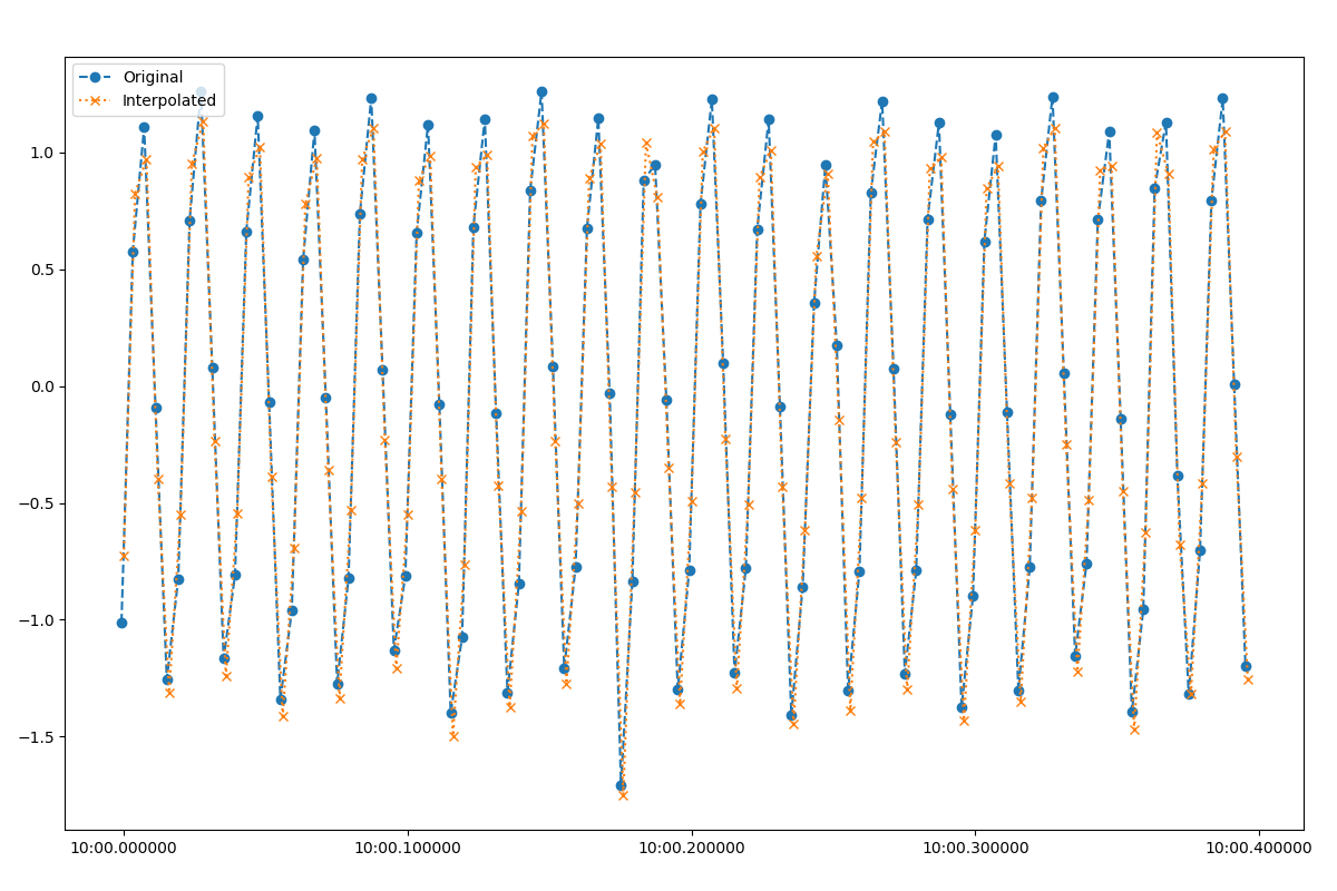
Original SPAM data versus interpolated data
Complete example script
For the purposes of clarity, the complete example script is shown below.
1 2 3 4 5 6 7 8 9 10 11 12 13 14 15 16 17 18 19 20 21 22 23 24 25 26 27 28 29 30 31 32 33 34 35 36 37 38 39 40 41 42 43 44 45 46 47 48 49 50 51 52 53 54 55 | from datapaths import timePath, timeImages
from resistics.time.reader_spam import TimeReaderSPAM
# read in spam data
spamPath = timePath / "spam"
spamReader = TimeReaderSPAM(spamPath)
spamReader.printInfo()
spamData = spamReader.getPhysicalSamples()
spamData.printInfo()
# interpolate to second
from resistics.time.interp import interpolateToSecond

interpData = interpolateToSecond(spamData, inplace=False)
interpData.printInfo()
# can now write out the interpolated dataset
from resistics.time.writer_internal import TimeWriterInternal

interpPath = timePath / "spamInterp"
headers = spamReader.getHeaders()
chanHeaders, chanMap = spamReader.getChanHeaders()
writer = TimeWriterInternal()
writer.setOutPath(interpPath)
writer.writeData(
    headers,
    chanHeaders,
    interpData,
    physical=True,
)
writer.printInfo()
# read in the internal data
from resistics.time.reader_internal import TimeReaderInternal

interpReader = TimeReaderInternal(interpPath)
interpReader.printInfo()
interpReader.printComments()
# get data between a time range
startTime = "2016-02-07 02:10:00"
stopTime = "2016-02-07 02:30:00"
spamData = spamReader.getPhysicalData(startTime, stopTime)
interpData = interpReader.getPhysicalData(startTime, stopTime)
# plot the datasets
import matplotlib.pyplot as plt

fig = plt.figure(figsize=(12, 8))
plt.plot(spamData.getDateArray()[0:100], spamData.data["Ex"][0:100], "o--")
plt.plot(interpData.getDateArray()[0:100], interpData.data["Ex"][0:100], "x:")
plt.legend(["Original", "Interpolated"], loc=2)
fig.tight_layout(rect=[0, 0.02, 1, 0.96])
plt.show()
fig.savefig(timeImages / "interpolation.png")
|