ASCII Calibration
The internal ASCII calibration format is a simple ASCII format meant to be used when no other format is available. Each file only contains one set of calibration data (no chopper on or off) and there is no provision for different chopper on and off files.
The units of the internal format ASCII calibration files are interpreted to be:
Frequency in Hz
Magnitude in mV/nT
Phase in degrees or radians depending on the “Phase unit” header
Resistics will automatically convert these units to:
Frequency in Hz
Magnitude in mV/nT (including any static gain)
Phase in radians
Naming in the project environment
When using the project environment, resistics automatically searches for calibration files in the calData folder. Internal format ASCII files should be named according to the following specification:
Important
[*]IC_[SERIAL].txt
where,
SERIAL is the sensor serial number
[*] represents any general string
As an example, consider an induction coil with:
sensor serial number 307
Then the file should be named:
IC_307.TXT
Or with any leading text, e.g. magcal_IC_307.TXT
As can be seen, there is no ability to distinguish different sensors with the same serial number or situations where chopper is on or off. For those cases, RSP or Metronix formats are better.
Example
The internal ASCII format calibration file will not usually be provided and will have to be created from scratch. The CalibrationIO class provides the handy writeInternalTemplate() method for producing a template internal ASCII format calibration file. A template can be made as follows:
1 2 3 4 5 6 7 | from datapaths import calPath, calImages
from resistics.calibrate.io import CalibrationIO
# we can write a template into which to paste our data
writepath = calPath / "ascii.txt"
calIO = CalibrationIO()
calIO.writeInternalTemplate(writepath, 307, "MFS06", 1)
|
This produces an empty calibration file with some basic information in:
1 2 3 4 5 6 7 8 | Serial = 307
Sensor = MFS06
Static gain = 1
Magnitude unit = mV/nT
Phase unit = degrees
Chopper = False
CALIBRATION DATA
|
The basic metadata can either be corrected in the file or passed as keywords to writeInternalTemplate(). The actual calibration data needs to be copied in and should be in the units:
Magnitude in mV/nT without static gain
Phase in units which match the “Phase unit” header, which can either be degrees or radians
An example file with calibration data copied is provided below.
1 2 3 4 5 6 7 8 9 10 11 12 13 14 15 16 17 18 19 20 21 22 23 24 25 26 27 28 29 30 31 32 33 34 35 36 37 38 39 | Serial = 307
Sensor = MFS06
Static gain = 1
Magnitude unit = mV/nT
Phase unit = radians
Chopper = False
CALIBRATION DATA
+1.0000e-01 +1.9967e+01 +1.5452e+00
+1.4678e-01 +2.9303e+01 +1.5339e+00
+2.1544e-01 +4.2933e+01 +1.5173e+00
+3.1623e-01 +6.2901e+01 +1.4931e+00
+4.6416e-01 +9.1945e+01 +1.4576e+00
+6.8130e-01 +1.3418e+02 +1.4051e+00
+1.0000e+00 +1.9404e+02 +1.3394e+00
+1.4678e+00 +2.7551e+02 +1.2296e+00
+2.1544e+00 +3.8111e+02 +1.0904e+00
+3.1623e+00 +5.0078e+02 +9.1815e-01
+4.6416e+00 +6.1636e+02 +7.2902e-01
+6.8130e+00 +7.0664e+02 +5.4810e-01
+1.0000e+01 +7.6400e+02 +3.9286e-01
+1.4678e+01 +7.9669e+02 +2.7489e-01
+2.1545e+01 +8.1231e+02 +1.8837e-01
+3.1623e+01 +8.2062e+02 +1.2735e-01
+4.6416e+01 +8.2453e+02 +8.4177e-02
+6.8130e+01 +8.2219e+02 +4.5146e-02
+1.0000e+02 +8.2609e+02 +2.8629e-02
+1.4678e+02 +8.2567e+02 +1.0910e-02
+2.1545e+02 +8.2660e+02 -7.6749e-03
+3.1623e+02 +8.2631e+02 -2.6356e-02
+4.6417e+02 +8.2636e+02 -4.8977e-02
+6.8130e+02 +8.2730e+02 -7.8009e-02
+1.0000e+03 +8.2795e+02 -1.2135e-01
+1.4678e+03 +8.2721e+02 -1.8637e-01
+2.1545e+03 +8.1548e+02 -2.8374e-01
+3.1623e+03 +7.9639e+02 -4.2317e-01
+4.6417e+03 +7.1928e+02 -6.2696e-01
+6.8130e+03 +6.1971e+02 -7.4339e-01
+1.0000e+04 +5.7145e+02 -9.7107e-01
|
This internal format ASCII calibration file can now be read in using the CalibrationIO class. First, the reading parameters need to be reset using the refresh() method. Using the read() method will return a CalibrationData object.
9 10 11 12 13 | # read back the internal template file
filepath = calPath / "asciiWithData.txt"
calIO.refresh(filepath, "induction", extend=False)
calData = calIO.read()
calData.printInfo()
|
The printInfo() method prints information about the calibration data.
1 2 3 4 5 6 7 8 9 10 11 12 13 14 15 16 17 18 19 20 21 22 23 24 25 26 27 28 29 30 31 32 33 34 35 36 37 38 39 40 41 42 43 44 45 | 15:15:46 CalibrationData: ####################
15:15:46 CalibrationData: CALIBRATIONDATA INFO BEGIN
15:15:46 CalibrationData: ####################
15:15:46 CalibrationData: Filename = calData\asciiWithData.txt
15:15:46 CalibrationData: Serial = 307
15:15:46 CalibrationData: Sensor = MFS06
15:15:46 CalibrationData: Static gain = 1.00
15:15:46 CalibrationData: Chopper = False
15:15:46 CalibrationData: Number of frequency points = 31
15:15:46 CalibrationData: Calibration data:
15:15:46 CalibrationData: Frequency [Hz] Mag. [mv/nT] Phase [rad]
15:15:46 CalibrationData: 0.10000000 19.97 1.55
15:15:46 CalibrationData: 0.14678000 29.30 1.53
15:15:46 CalibrationData: 0.21544000 42.93 1.52
15:15:46 CalibrationData: 0.31623000 62.90 1.49
15:15:46 CalibrationData: 0.46416000 91.94 1.46
15:15:46 CalibrationData: 0.68130000 134.18 1.41
15:15:46 CalibrationData: 1.00000000 194.04 1.34
15:15:46 CalibrationData: 1.46780000 275.51 1.23
15:15:46 CalibrationData: 2.15440000 381.11 1.09
15:15:46 CalibrationData: 3.16230000 500.78 0.92
15:15:46 CalibrationData: 4.64160000 616.36 0.73
15:15:46 CalibrationData: 6.81300000 706.64 0.55
15:15:46 CalibrationData: 10.00000000 764.00 0.39
15:15:46 CalibrationData: 14.67800000 796.69 0.27
15:15:46 CalibrationData: 21.54500000 812.31 0.19
15:15:46 CalibrationData: 31.62300000 820.62 0.13
15:15:46 CalibrationData: 46.41600000 824.53 0.08
15:15:46 CalibrationData: 68.13000000 822.19 0.05
15:15:46 CalibrationData: 100.00000000 826.09 0.03
15:15:46 CalibrationData: 146.78000000 825.67 0.01
15:15:46 CalibrationData: 215.45000000 826.60 -0.01
15:15:46 CalibrationData: 316.23000000 826.31 -0.03
15:15:46 CalibrationData: 464.17000000 826.36 -0.05
15:15:46 CalibrationData: 681.30000000 827.30 -0.08
15:15:46 CalibrationData: 1000.00000000 827.95 -0.12
15:15:46 CalibrationData: 1467.80000000 827.21 -0.19
15:15:46 CalibrationData: 2154.50000000 815.48 -0.28
15:15:46 CalibrationData: 3162.30000000 796.39 -0.42
15:15:46 CalibrationData: 4641.70000000 719.28 -0.63
15:15:46 CalibrationData: 6813.00000000 619.71 -0.74
15:15:46 CalibrationData: 10000.00000000 571.45 -0.97
15:15:46 CalibrationData: ####################
15:15:46 CalibrationData: CALIBRATIONDATA INFO END
15:15:46 CalibrationData: ####################
|
To view the calibration data, the view() method of CalibrationData can be used. By passing a matplotlib figure to this, the layout of the plot can be controlled.
15 16 17 18 19 20 21 22 | # plot
import matplotlib.pyplot as plt
fig = plt.figure(figsize=(8, 8))
calData.view(fig=fig, label="Internal ASCII format", legend=True)
fig.tight_layout(rect=[0, 0.02, 1, 0.96])
plt.show()
fig.savefig(calImages / "calibrationASCII.png")
|
This produces the following plot:
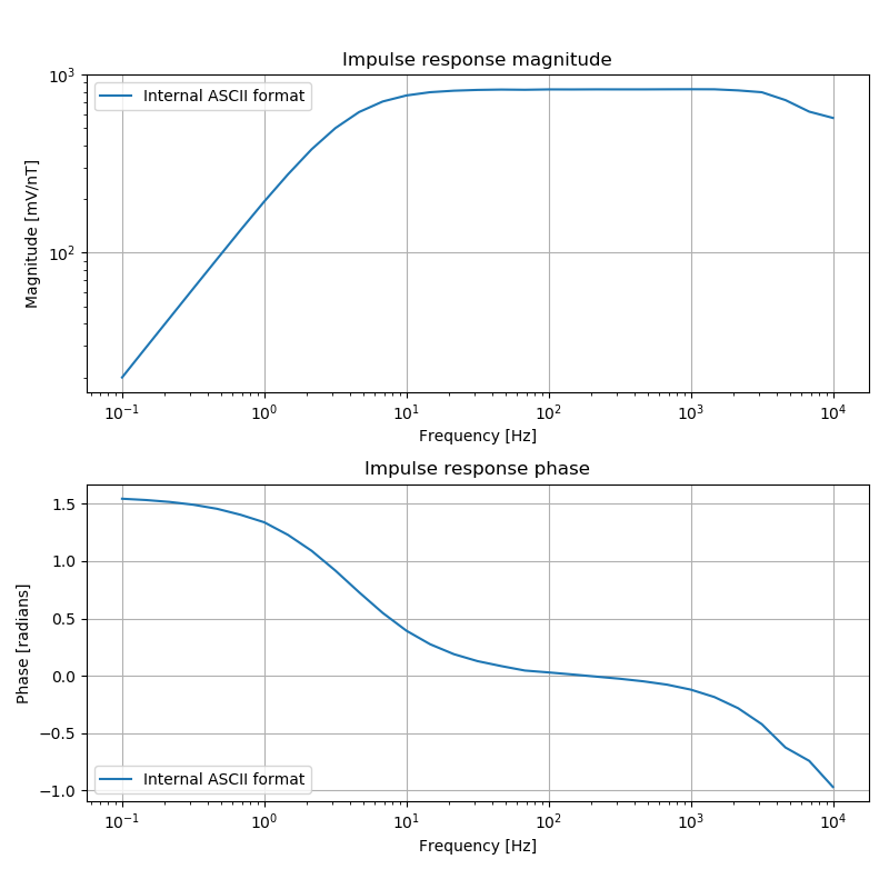
Viewing the unextended calibration data from the internal format ASCII file
Complete example script
For the purposes of clarity, the example script in full.
1 2 3 4 5 6 7 8 9 10 11 12 13 14 15 16 17 18 19 20 21 22 | from datapaths import calPath, calImages
from resistics.calibrate.io import CalibrationIO
# we can write a template into which to paste our data
writepath = calPath / "ascii.txt"
calIO = CalibrationIO()
calIO.writeInternalTemplate(writepath, 307, "MFS06", 1)
# read back the internal template file
filepath = calPath / "asciiWithData.txt"
calIO.refresh(filepath, "induction", extend=False)
calData = calIO.read()
calData.printInfo()
# plot
import matplotlib.pyplot as plt

fig = plt.figure(figsize=(8, 8))
calData.view(fig=fig, label="Internal ASCII format", legend=True)
fig.tight_layout(rect=[0, 0.02, 1, 0.96])
plt.show()
fig.savefig(calImages / "calibrationASCII.png")
|
1 2 3 4 5 6 7 8 9 10 11 12 13 14 15 16 17 18 19 20 21 22 23 24 25 26 27 28 29 30 31 32 33 34 35 36 37 38 39 | Serial = 307
Sensor = MFS06
Static gain = 1
Magnitude unit = mV/nT
Phase unit = radians
Chopper = False
CALIBRATION DATA
+1.0000e-01 +1.9967e+01 +1.5452e+00
+1.4678e-01 +2.9303e+01 +1.5339e+00
+2.1544e-01 +4.2933e+01 +1.5173e+00
+3.1623e-01 +6.2901e+01 +1.4931e+00
+4.6416e-01 +9.1945e+01 +1.4576e+00
+6.8130e-01 +1.3418e+02 +1.4051e+00
+1.0000e+00 +1.9404e+02 +1.3394e+00
+1.4678e+00 +2.7551e+02 +1.2296e+00
+2.1544e+00 +3.8111e+02 +1.0904e+00
+3.1623e+00 +5.0078e+02 +9.1815e-01
+4.6416e+00 +6.1636e+02 +7.2902e-01
+6.8130e+00 +7.0664e+02 +5.4810e-01
+1.0000e+01 +7.6400e+02 +3.9286e-01
+1.4678e+01 +7.9669e+02 +2.7489e-01
+2.1545e+01 +8.1231e+02 +1.8837e-01
+3.1623e+01 +8.2062e+02 +1.2735e-01
+4.6416e+01 +8.2453e+02 +8.4177e-02
+6.8130e+01 +8.2219e+02 +4.5146e-02
+1.0000e+02 +8.2609e+02 +2.8629e-02
+1.4678e+02 +8.2567e+02 +1.0910e-02
+2.1545e+02 +8.2660e+02 -7.6749e-03
+3.1623e+02 +8.2631e+02 -2.6356e-02
+4.6417e+02 +8.2636e+02 -4.8977e-02
+6.8130e+02 +8.2730e+02 -7.8009e-02
+1.0000e+03 +8.2795e+02 -1.2135e-01
+1.4678e+03 +8.2721e+02 -1.8637e-01
+2.1545e+03 +8.1548e+02 -2.8374e-01
+3.1623e+03 +7.9639e+02 -4.2317e-01
+4.6417e+03 +7.1928e+02 -6.2696e-01
+6.8130e+03 +6.1971e+02 -7.4339e-01
+1.0000e+04 +5.7145e+02 -9.7107e-01
|