RSP Calibration
RSP calibration files are ASCII files with metadata and calibration data.
The units of RSP calibration files are interpreted to be:
Frequency in Hz
Magnitude in mV/nT
Phase in degrees
Resistics will automatically convert these units to:
Frequency in Hz
Magnitude in mV/nT (including any static gain)
Phase in radians
Note
Remember that extension happens in the original units of the calibration data. For RSP data files, this is in mV/nT.
Naming in the project environment
When using the project environment, resistics automatically searches for calibration files in the calData folder. RSP files should be named according to the following specification:
Important
[*]TYPE-[SENSORNUM]_[BOARD]-ID-[SERIAL].RSP
or
[*]TYPE-[SENSORNUM]_BB-ID-[SERIAL].RSP
where:
SENSORNUM is the sensor number out of the sensor type written with three digits (i.e. leading zeros required if the sensor number is less than three digits)
BOARD is either LF (chopper on) or HF (chopper off)
SERIAL is the serial number written with six digits (i.e. leading zeros required if the serial number is less than six digits)
[*] represents any general string.
The BB files represent broadband calibration files that cover both chopper on and chopper off cases.
As an example, consider an induction coil with,
sensor type MFS06
sensor serial number 307
Chopper off
then,
SENSORNUM = 006
BOARD = HF
SERIAL = 000307
Therefore, the file could be named:
Metronix_Coil—–TYPE-006_HF-ID-000307.RSP
Metronix_Coil—–TYPE-006_BB-ID-000307.RSP
Example
The class CalibrationIO can be used to read in RSP calibration files.
1 2 3 4 5 6 7 8 | from datapaths import calPath, calImages
from resistics.calibrate.io import CalibrationIO
# read RSP calibration data - this is a broadband calibraition - no chopper on or off
filepath = calPath / "Metronix_Coil-----TYPE-006_BB-ID-000307.RSP"
calIO = CalibrationIO(filepath, "rsp", extend=False)
calData = calIO.read()
calData.printInfo()
|
When using CalibrationIO to read a calibration file, the filepath and calibration data format (rsp) need to be defined. Further, the extension rule can be optionally passed. Because RSP files only contain one set of calibration data (unlike Metronix files which may have calibration data for both chopper on and off), the chopper keyword is unused for reading RSP files.
The method read() returns a CalibrationData object. Information about this can be printed to the terminal, giving:
1 2 3 4 5 6 7 8 9 10 11 12 13 14 15 16 17 18 19 20 21 22 23 24 25 26 27 28 29 30 31 32 33 34 35 36 37 38 39 40 41 42 43 44 45 46 47 48 49 50 51 52 53 54 | 14:10:49 CalibrationData: ####################
14:10:49 CalibrationData: CALIBRATIONDATA INFO BEGIN
14:10:49 CalibrationData: ####################
14:10:49 CalibrationData: Filename = calData\Metronix_Coil-----TYPE-006_BB-ID-000307.RSP
14:10:49 CalibrationData: Serial = 307
14:10:49 CalibrationData: Sensor = 006_HF
14:10:49 CalibrationData: Static gain = 800.00
14:10:49 CalibrationData: Chopper = False
14:10:49 CalibrationData: Number of frequency points = 40
14:10:49 CalibrationData: Calibration data:
14:10:49 CalibrationData: Frequency [Hz] Mag. [mv/nT] Phase [rad]
14:10:49 CalibrationData: 0.00001000 0.00 1.57
14:10:49 CalibrationData: 0.00010000 0.02 1.57
14:10:49 CalibrationData: 0.00100000 0.20 1.57
14:10:49 CalibrationData: 0.01000000 2.00 1.57
14:10:49 CalibrationData: 0.02000000 4.00 1.57
14:10:49 CalibrationData: 0.03000000 6.00 1.56
14:10:49 CalibrationData: 0.04000000 8.00 1.56
14:10:49 CalibrationData: 0.05000000 10.00 1.56
14:10:49 CalibrationData: 0.07000000 14.00 1.55
14:10:49 CalibrationData: 0.10000000 19.97 1.55
14:10:49 CalibrationData: 0.14678000 29.30 1.53
14:10:49 CalibrationData: 0.21544000 42.93 1.52
14:10:49 CalibrationData: 0.31623000 62.90 1.49
14:10:49 CalibrationData: 0.46416000 91.95 1.46
14:10:49 CalibrationData: 0.68130000 134.18 1.41
14:10:49 CalibrationData: 1.00000000 194.04 1.34
14:10:49 CalibrationData: 1.46780000 275.51 1.23
14:10:49 CalibrationData: 2.15440000 381.11 1.09
14:10:49 CalibrationData: 3.16230000 500.78 0.92
14:10:49 CalibrationData: 4.64160000 616.36 0.73
14:10:49 CalibrationData: 6.81300000 706.64 0.55
14:10:49 CalibrationData: 10.00000000 764.00 0.39
14:10:49 CalibrationData: 14.67800000 796.69 0.27
14:10:49 CalibrationData: 21.54500000 812.31 0.19
14:10:49 CalibrationData: 31.62300000 820.62 0.13
14:10:49 CalibrationData: 46.41600000 824.53 0.08
14:10:49 CalibrationData: 68.13000000 822.19 0.05
14:10:49 CalibrationData: 100.00000000 826.09 0.03
14:10:49 CalibrationData: 146.78000000 827.91 0.01
14:10:49 CalibrationData: 215.45000000 827.59 -0.01
14:10:49 CalibrationData: 316.23000000 827.04 -0.03
14:10:49 CalibrationData: 464.16000000 827.32 -0.05
14:10:49 CalibrationData: 681.30000000 828.12 -0.08
14:10:49 CalibrationData: 1000.00000000 829.22 -0.12
14:10:49 CalibrationData: 1467.80000000 828.29 -0.19
14:10:49 CalibrationData: 2154.50000000 816.08 -0.28
14:10:49 CalibrationData: 3162.30000000 797.63 -0.42
14:10:49 CalibrationData: 4641.70000000 720.48 -0.63
14:10:49 CalibrationData: 6813.00000000 619.91 -0.74
14:10:49 CalibrationData: 10000.00000000 571.23 -0.97
14:10:49 CalibrationData: ####################
14:10:49 CalibrationData: CALIBRATIONDATA INFO END
14:10:49 CalibrationData: ####################
|
Once the calibration data file is read in, the calibration curve can be viewed by using the view() method of CalibrationData. By passing a matplotlib figure to this, the layout of the plot can be controlled.
10 11 12 13 14 15 16 17 | # plot
import matplotlib.pyplot as plt
fig = plt.figure(figsize=(8, 8))
calData.view(fig=fig, label="RSP calibration", legend=True)
fig.tight_layout(rect=[0, 0.02, 1, 0.96])
plt.show()
fig.savefig(calImages / "calibrationRSP.png")
|
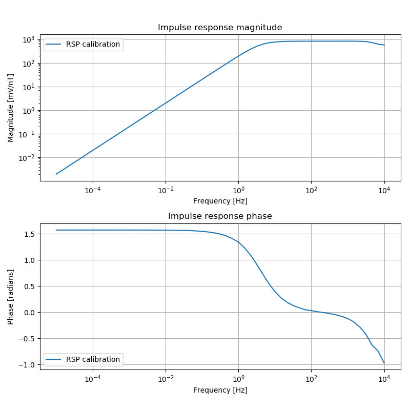
Viewing the unextended calibration data
The calibration static gain is applied to the magnitude data by default. To view the data without static gain, pass staticgain=False to the view() call. Further, to plot the phase in degrees, pass degrees=True to view().
To visualise the influence of the static gain correction, the calibration data can be plotted with and without static gain as shown in the following example.
19 20 21 22 23 24 25 26 27 28 29 | # plot
import matplotlib.pyplot as plt
fig = plt.figure(figsize=(8, 8))
calData.view(fig=fig, label="RSP calibration", degrees=True, legend=True)
calData.view(
fig=fig, staticgain=False, degrees=True, label="RSP no static gain", legend=True
)
fig.tight_layout(rect=[0, 0.02, 1, 0.96])
plt.show()
fig.savefig(calImages / "calibrationRSP_staticGainAndDegrees.png")
|
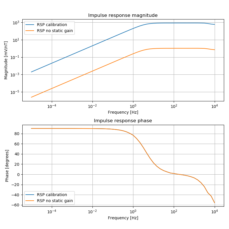
Viewing the unextended calibration data with and without static gain
The calibration data can be written out in the internal ASCII format using the writeInternalFormat() method of CalibrationIO.
31 32 33 | # write as the ASCII format
rsp2ascii = calPath / "rsp2ascii.TXT"
calIO.writeInternalFormat(calData, rsp2ascii)
|
The internal ascii calibration format writes out values in the following units:
Magnitude in mV/nT
Phase in radians
This gives the file below:
1 2 3 4 5 6 7 8 9 10 11 12 13 14 15 16 17 18 19 20 21 22 23 24 25 26 27 28 29 30 31 32 33 34 35 36 37 38 39 40 41 42 43 44 45 46 47 48 | Serial = 307
Sensor = 006_HF
Static gain = 800.0
Magnitude unit = mV/nT
Phase unit = radians
Chopper = False
CALIBRATION DATA
+1.0000e-05 +2.5000e-06 +1.5708e+00
+1.0000e-04 +2.5000e-05 +1.5708e+00
+1.0000e-03 +2.5000e-04 +1.5705e+00
+1.0000e-02 +2.5000e-03 +1.5683e+00
+2.0000e-02 +4.9999e-03 +1.5658e+00
+3.0000e-02 +7.4998e-03 +1.5633e+00
+4.0000e-02 +9.9995e-03 +1.5608e+00
+5.0000e-02 +1.2499e-02 +1.5583e+00
+7.0000e-02 +1.7497e-02 +1.5533e+00
+1.0000e-01 +2.4959e-02 +1.5452e+00
+1.4678e-01 +3.6629e-02 +1.5339e+00
+2.1544e-01 +5.3666e-02 +1.5173e+00
+3.1623e-01 +7.8627e-02 +1.4931e+00
+4.6416e-01 +1.1493e-01 +1.4576e+00
+6.8130e-01 +1.6773e-01 +1.4051e+00
+1.0000e+00 +2.4255e-01 +1.3394e+00
+1.4678e+00 +3.4438e-01 +1.2296e+00
+2.1544e+00 +4.7639e-01 +1.0904e+00
+3.1623e+00 +6.2598e-01 +9.1815e-01
+4.6416e+00 +7.7045e-01 +7.2902e-01
+6.8130e+00 +8.8331e-01 +5.4810e-01
+1.0000e+01 +9.5500e-01 +3.9286e-01
+1.4678e+01 +9.9587e-01 +2.7489e-01
+2.1545e+01 +1.0154e+00 +1.8837e-01
+3.1623e+01 +1.0258e+00 +1.2735e-01
+4.6416e+01 +1.0307e+00 +8.4177e-02
+6.8130e+01 +1.0277e+00 +4.5146e-02
+1.0000e+02 +1.0326e+00 +2.8629e-02
+1.4678e+02 +1.0349e+00 +7.9399e-03
+2.1545e+02 +1.0345e+00 -7.9172e-03
+3.1623e+02 +1.0338e+00 -2.6454e-02
+4.6416e+02 +1.0341e+00 -4.8852e-02
+6.8130e+02 +1.0352e+00 -7.9795e-02
+1.0000e+03 +1.0365e+00 -1.2133e-01
+1.4678e+03 +1.0354e+00 -1.8783e-01
+2.1545e+03 +1.0201e+00 -2.8487e-01
+3.1623e+03 +9.9703e-01 -4.2295e-01
+4.6417e+03 +9.0061e-01 -6.2766e-01
+6.8130e+03 +7.7489e-01 -7.4444e-01
+1.0000e+04 +7.1404e-01 -9.7162e-01
|
Note
When writing out in internal format, the static gain is removed from the magnitude but recorded in the file. When reading in the internal format again, the static gain will be reapplied.
To read in the internal ASCII format calibration file, the parameters of CalibrationIO need to be reset using the refresh() method. This time, the fileformat needs to be set to “induction”.
35 36 37 38 | # can read this again
calIO.refresh(rsp2ascii, "induction", extend=False)
calDataAscii = calIO.read()
calDataAscii.printInfo()
|
Finally, plotting the original data and the internal ASCII format data can be done in the following way:
40 41 42 43 44 45 46 | # plot together
fig = plt.figure(figsize=(8, 8))
calData.view(fig=fig, label="RSP calibration", legend=True)
calDataAscii.view(fig=fig, label="ASCII calibration", legend=True)
fig.tight_layout(rect=[0, 0.02, 1, 0.96])
plt.show()
fig.savefig(calImages / "calibrationRSPvsASCII.png")
|
The resultant figure is:
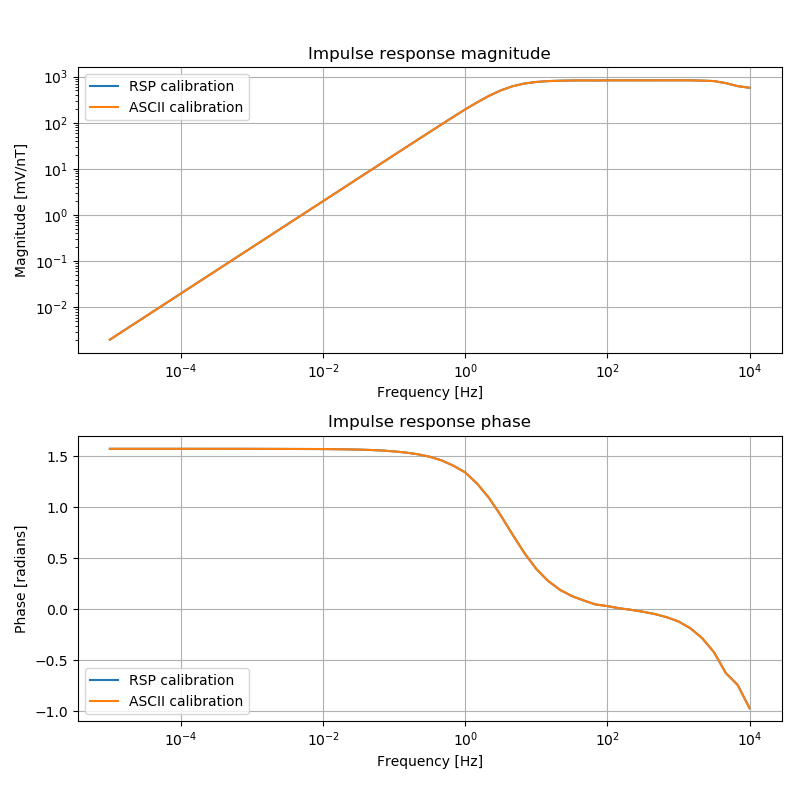
Viewing the original RSP data versus the ASCII data
Complete example script
For the purposes of clarity, the example script in full.
1 2 3 4 5 6 7 8 9 10 11 12 13 14 15 16 17 18 19 20 21 22 23 24 25 26 27 28 29 30 31 32 33 34 35 36 37 38 39 40 41 42 43 44 45 46 | from datapaths import calPath, calImages
from resistics.calibrate.io import CalibrationIO
# read RSP calibration data - this is a broadband calibraition - no chopper on or off
filepath = calPath / "Metronix_Coil-----TYPE-006_BB-ID-000307.RSP"
calIO = CalibrationIO(filepath, "rsp", extend=False)
calData = calIO.read()
calData.printInfo()
# plot
import matplotlib.pyplot as plt

fig = plt.figure(figsize=(8, 8))
calData.view(fig=fig, label="RSP calibration", legend=True)
fig.tight_layout(rect=[0, 0.02, 1, 0.96])
plt.show()
fig.savefig(calImages / "calibrationRSP.png")
# plot
import matplotlib.pyplot as plt

fig = plt.figure(figsize=(8, 8))
calData.view(fig=fig, label="RSP calibration", degrees=True, legend=True)
calData.view(
    fig=fig, staticgain=False, degrees=True, label="RSP no static gain", legend=True
)
fig.tight_layout(rect=[0, 0.02, 1, 0.96])
plt.show()
fig.savefig(calImages / "calibrationRSP_staticGainAndDegrees.png")
# write as the ASCII format
rsp2ascii = calPath / "rsp2ascii.TXT"
calIO.writeInternalFormat(calData, rsp2ascii)
# can read this again
calIO.refresh(rsp2ascii, "induction", extend=False)
calDataAscii = calIO.read()
calDataAscii.printInfo()
# plot together
fig = plt.figure(figsize=(8, 8))
calData.view(fig=fig, label="RSP calibration", legend=True)
calDataAscii.view(fig=fig, label="ASCII calibration", legend=True)
fig.tight_layout(rect=[0, 0.02, 1, 0.96])
plt.show()
fig.savefig(calImages / "calibrationRSPvsASCII.png")
|
1 2 3 4 5 6 7 8 9 10 11 12 13 14 15 16 17 18 19 20 21 22 23 24 25 26 27 28 29 30 31 32 33 34 35 36 37 38 39 40 41 42 43 44 45 46 47 48 49 50 51 52 53 54 55 56 57 58 59 60 61 62 63 64 65 66 67 68 69 | Info MFS06 induction coil no.: 365 - date of calibration: Nov 2012
Info BB - files HF and LF put together
Info theoretical values used for f less than 0.1Hz
StaticGain 800.00000000
CalFile
Manufacturer Metronix_Coil-----
SensorType 006_HF
FREQUENCY(Hz) AMPLITUDE(mV/nT) PHASE(deg)
--------------------------------------------------
10000.00000000 0.68111250 -55.00600000
7943.00000000 0.71691532 -47.00600000
6309.40000000 0.75118139 -42.80600000
5011.80000000 0.84298476 -39.21300000
3981.00000000 0.92956350 -32.18700000
3162.20000000 0.97526201 -25.51500000
2511.80000000 1.00296174 -20.14600000
1995.20000000 1.01615536 -15.37100000
1584.90000000 1.02166616 -12.19400000
1258.90000000 1.02757713 -9.60450000
1000.00000000 1.02927500 -7.41570000
794.30000000 1.03139855 -5.99240000
630.95000000 1.03286515 -4.61200000
501.18000000 1.03280668 -3.47730000
398.10000000 1.03441309 -2.62020000
316.22000000 1.03419751 -1.80970000
251.19000000 1.03452602 -1.18630000
199.52000000 1.03448626 -0.43138000
158.49000000 1.03713875 0.00156320
125.89000000 1.03530362 0.84879000
100.00000000 1.03295000 1.56090000
79.43000000 1.03249071 2.38410000
63.09500000 1.03680859 3.30920000
50.11800000 1.02867195 4.44710000
39.81000000 1.02590370 5.50290000
31.62200000 1.02609437 7.09880000
25.11900000 1.01870105 9.11900000
19.95200000 1.01256400 11.53900000
15.84900000 1.00064643 14.52300000
12.58900000 0.98378314 18.15600000
10.00000000 0.95576250 22.41100000
7.94300000 0.91780372 27.48100000
6.30950000 0.86550566 33.02300000
5.01180000 0.79844239 39.38100000
3.98100000 0.71901836 46.10100000
3.16230000 0.62751891 52.42100000
2.51190000 0.53698142 58.62300000
1.99520000 0.44989266 64.07800000
1.58490000 0.37068830 68.95500000
1.25890000 0.30175833 72.91200000
1.00000000 0.24387500 76.25400000
0.79430000 0.19548716 78.95400000
0.63095000 0.15654658 81.02300000
0.50119000 0.12492161 82.91800000
0.39811000 0.09926375 84.36700000
0.31623000 0.07913260 85.55200000
0.25119000 0.06284774 86.40200000
0.19953000 0.04990994 87.11700000
0.15849000 0.03965618 87.66700000
0.12589000 0.03152600 88.16100000
0.10000000 0.02505375 88.52000000
0.07000000 0.01749732 88.99693298
0.05000000 0.01249902 89.28348541
0.04000000 0.00999950 89.42677307
0.03000000 0.00749979 89.57008362
0.02000000 0.00499994 89.71337891
0.01000000 0.00249999 89.85668945
0.00100000 0.00025000 89.98566437
0.00010000 0.00002500 89.99856567
0.00001000 0.00000250 89.99985504
|