Remote reference processing
Remote reference processing can help achieve notably better transfer functions in the presence of electromagnetic (EM) noise or when the signal to noise ratio within the magnetotelluric deadband is poor. To be able to perform remote reference processing, the following is required:
The local site and the remote site must be at the same sampling frequency
The local site and remote site must have a period of time with concurrent recording
The example here will deal with following:
A local site recorded in northern Switzerland in 2016 and named M6. The sampling frequencys recorded at M6 include 65536, 16384, 4096, 512 and 128 Hz. The sampling frequency of interest for remote reference processing is 128 Hz and the format is ATS.
A remote site permanently stationed in Germany. The sampling frequency of this data is 250 Hz and the format is SPAM. The site for the remote reference SPAM data will be called RemoteSPAM.
Magnetotelluric data from northern Switzerland is noisy, particularly in the dead band due to the poor signal to noise ratio when accouting for the environmental noise, but at other evaluation frequencies too. Further, there is biasing and coherent sources of eletromagnetic noise. The hope is to use remote reference processing to help improve the impedance tensor estimates.
Setting up the project
Begin as usual by creating our project and two sites to put our data in.
1 2 3 4 5 6 7 8 9 10 11 | from datapaths import remotePath
from resistics.project.io import newProject
# define the project path. The project will be created under this project path.
# If the path does not exist, it will be created
projData = newProject(remotePath, "2016-01-18 00:00:00")
# let's create 2 sites
# M6 is the location of interest. Remote is a remote reference station.
projData.createSite("M6")
projData.createSite("RemoteSPAM")
|
After placing the data in the relevant folders, the project looks like this:
exampleProject
├── calData
├── timeData
│   |── M6
|   |   |── meas_2016-02-15_15-00-03
│   |   |── meas_2016-02-15_15-02-03
|   |   |── meas_2016-02-15_15-04-03
|   |   |── meas_2016-02-15_15-08-03
|   |   |── meas_2016-02-15_15-08-03
|   |   |── meas_2016-02-15_15-08-03
|   |   |── meas_2016-02-15_15-08-03
|   |   |── meas_2016-02-15_15-28-06
|   |   |── meas_2016-02-16_02-00-00
|   |   |── meas_2016-02-16_02-35-00
|   |   |── meas_2016-02-17_02-00-00
|   |   |── meas_2016-02-17_02-35-00
|   |   |── meas_2016-02-18_02-00-00
|   |   |── meas_2016-02-18_02-35-00
|   |   |── meas_2016-02-19_02-00-00
|   |   |── meas_2016-02-19_02-35-00
|   |   |── meas_2016-02-20_02-00-00
|   |   |── meas_2016-02-20_02-35-00
|   |   |── meas_2016-02-21_02-00-00
|   |   └── meas_2016-02-21_02-35-00
│   └── RemoteSPAM
|       └── run2
├── specData
├── statData
├── maskData
├── transFuncData
├── images
└── mtProj.prj
And printing out the project information and site information for the using shows the following result:
1 2 3 4 5 6 7 8 9 10 11 12 13 14 15 16 17 18 19 20 21 22 23 24 25 26 27 28 29 30 31 32 33 34 35 36 37 38 39 40 41 42 43 44 45 46 47 48 49 50 51 52 53 54 55 56 57 58 59 60 61 62 63 64 65 66 67 68 69 70 71 72 | 21:50:32 ProjectData: ####################
21:50:32 ProjectData: PROJECTDATA INFO BEGIN
21:50:32 ProjectData: ####################
21:50:32 ProjectData: Time data path = remoteProject\timeData
21:50:32 ProjectData: Spectra data path = remoteProject\specData
21:50:32 ProjectData: Statistics data path = remoteProject\statData
21:50:32 ProjectData: Mask data path = remoteProject\maskData
21:50:32 ProjectData: TransFunc data path = remoteProject\transFuncData
21:50:32 ProjectData: Calibration data path = remoteProject\calData
21:50:32 ProjectData: Images data path = remoteProject\images
21:50:32 ProjectData: Reference time = 2016-01-18 00:00:00
21:50:32 ProjectData: Project start time = 2016-02-11 00:00:00.003200
21:50:32 ProjectData: Project stop time = 2016-03-17 23:59:59.999200
21:50:32 ProjectData: Project found 2 sites:
21:50:32 ProjectData: M6 start: 2016-02-15 15:00:03 end: 2016-02-21 06:27:12.375000
21:50:32 ProjectData: RemoteSPAM start: 2016-02-11 00:00:00.003200 end: 2016-03-17 23:59:59.999200
21:50:32 ProjectData: Sampling frequencies found in project (Hz): 128.0, 250.0, 512.0, 4096.0, 16384.0, 65536.0
21:50:32 ProjectData: ####################
21:50:32 ProjectData: PROJECTDATA INFO END
21:50:32 ProjectData: ####################
22:00:30 SiteData: ####################
22:00:30 SiteData: SITEDATA INFO BEGIN
22:00:30 SiteData: ####################
22:00:30 SiteData: Site = M6
22:00:30 SiteData: Time data path = remoteProject\timeData\M6
22:00:30 SiteData: Spectra data path = remoteProject\specData\M6
22:00:30 SiteData: Statistics data path = remoteProject\statData\M6
22:00:30 SiteData: TransFunc data path = remoteProject\transFuncData\M6
22:00:30 SiteData: Site start time = 2016-02-15 15:00:03
22:00:30 SiteData: Site stop time = 2016-02-21 06:27:12.375000
22:00:30 SiteData: Sampling frequencies recorded = 128.00000000, 512.00000000, 4096.00000000, 16384.00000000, 65536.00000000
22:00:30 SiteData: Number of measurement files = 17
22:00:30 SiteData: Measurement Sample Frequency (Hz) Start Time End Time
22:00:30 SiteData: meas_2016-02-15_15-00-03 65536.0 2016-02-15 15:00:03 2016-02-15 15:01:02.999985
22:00:30 SiteData: meas_2016-02-15_15-02-03 16384.0 2016-02-15 15:02:03 2016-02-15 15:03:02.999939
22:00:30 SiteData: meas_2016-02-15_15-04-03 4096.0 2016-02-15 15:04:03 2016-02-15 15:07:02.999756
22:00:30 SiteData: meas_2016-02-15_15-08-03 512.0 2016-02-15 15:08:03 2016-02-15 15:13:02.998047
22:00:30 SiteData: meas_2016-02-15_15-28-06 128.0 2016-02-15 15:28:06 2016-02-16 01:54:59.992188
22:00:30 SiteData: meas_2016-02-16_02-00-00 4096.0 2016-02-16 02:00:00 2016-02-16 02:29:59.999756
22:00:30 SiteData: meas_2016-02-16_02-35-00 128.0 2016-02-16 02:35:00 2016-02-17 01:54:59.992188
22:00:30 SiteData: meas_2016-02-17_02-00-00 4096.0 2016-02-17 02:00:00 2016-02-17 02:29:59.999756
22:00:30 SiteData: meas_2016-02-17_02-35-00 128.0 2016-02-17 02:35:00 2016-02-18 01:54:59.992188
22:00:30 SiteData: meas_2016-02-18_02-00-00 4096.0 2016-02-18 02:00:00 2016-02-18 02:29:59.999756
22:00:30 SiteData: meas_2016-02-18_02-35-00 128.0 2016-02-18 02:35:00 2016-02-19 01:54:59.992188
22:00:30 SiteData: meas_2016-02-19_02-00-00 4096.0 2016-02-19 02:00:00 2016-02-19 02:29:59.999756
22:00:30 SiteData: meas_2016-02-19_02-35-00 128.0 2016-02-19 02:35:00 2016-02-20 01:54:59.992188
22:00:30 SiteData: meas_2016-02-20_02-00-00 4096.0 2016-02-20 02:00:00 2016-02-20 02:29:59.999756
22:00:30 SiteData: meas_2016-02-20_02-35-00 128.0 2016-02-20 02:35:00 2016-02-21 01:54:59.992188
22:00:30 SiteData: meas_2016-02-21_02-00-00 4096.0 2016-02-21 02:00:00 2016-02-21 02:29:59.999756
22:00:30 SiteData: meas_2016-02-21_02-35-00 128.0 2016-02-21 02:35:00 2016-02-21 06:27:12.375000
22:00:30 SiteData: ####################
22:00:30 SiteData: SITEDATA INFO END
22:00:30 SiteData: ####################
22:01:15 SiteData: ####################
22:01:15 SiteData: SITEDATA INFO BEGIN
22:01:15 SiteData: ####################
22:01:15 SiteData: Site = RemoteSPAM
22:01:15 SiteData: Time data path = remoteProject\timeData\RemoteSPAM
22:01:15 SiteData: Spectra data path = remoteProject\specData\RemoteSPAM
22:01:15 SiteData: Statistics data path = remoteProject\statData\RemoteSPAM
22:01:15 SiteData: TransFunc data path = remoteProject\transFuncData\RemoteSPAM
22:01:15 SiteData: Site start time = 2016-02-11 00:00:00.003200
22:01:15 SiteData: Site stop time = 2016-03-17 23:59:59.999200
22:01:15 SiteData: Sampling frequencies recorded = 250.00000000
22:01:15 SiteData: Number of measurement files = 1
22:01:15 SiteData: Measurement Sample Frequency (Hz) Start Time End Time
22:01:15 SiteData: run2 250.0 2016-02-11 00:00:00.003200 2016-03-17 23:59:59.999200
22:01:15 SiteData: ####################
22:01:15 SiteData: SITEDATA INFO END
22:01:15 SiteData: ####################
|
Pre-processing
As stated earlier, the project consists of:
local site M6 with several sampling frequencies
remote site RemoteSPAM with a single sampling frequency of 250 Hz
Recall, the remote data will be used as a remote reference for the 128 Hz data at local site M6. Therefore, the first step is to pre-process the remote data (for more information about pre-processing in resistics, see Pre-processing timeseries data). For SPAM data, this means:
Interpolation on to the second
Resampling to 128 Hz
As usual, the project is loaded in. Information is printed out about each site and then the remote reference data is pre-processed using the preprocess() method.
1 2 3 4 5 6 7 8 9 10 11 12 13 14 15 16 17 18 19 20 21 22 23 24 25 26 27 28 29 30 31 32 33 34 | from datapaths import remotePath, remoteImages
from resistics.project.io import loadProject
from resistics.project.time import preProcess, viewTime
proj = loadProject(remotePath)
proj.printInfo()
# get information about the local site
siteLocal = proj.getSiteData("M6")
siteLocal.printInfo()
# get information about the SPAM data remote reference
siteRemote = proj.getSiteData("RemoteSPAM")
siteRemote.printInfo()
# want to resample the RemoteSPAM data to 128 Hz
# SPAM data want to resample onto the second
# to make sure the times are matching, we can loop through the 128Hz measurements of M6 and use those times
meas128 = siteLocal.getMeasurements(128)
for meas in meas128:
start = siteLocal.getMeasurementStart(meas).strftime("%Y-%m-%d %H:%M:%S")
stop = siteLocal.getMeasurementEnd(meas).strftime("%Y-%m-%d %H:%M:%S")
postpend = siteLocal.getMeasurementStart(meas).strftime("%Y-%m-%d_%H-%M-%S")
print("Processing data from {} to {}".format(start, stop))
preProcess(
proj,
sites="RemoteSPAM",
start=start,
stop=stop,
interp=True,
resamp={250: 128},
outputsite="Remote",
prepend="",
postpend=postpend,
)
proj.refresh()
|
Of particular interest is this part of the of the process:
14 15 16 17 18 19 20 21 22 23 24 25 26 27 28 29 30 31 32 33 34 | # want to resample the RemoteSPAM data to 128 Hz
# SPAM data want to resample onto the second
# to make sure the times are matching, we can loop through the 128Hz measurements of M6 and use those times
meas128 = siteLocal.getMeasurements(128)
for meas in meas128:
start = siteLocal.getMeasurementStart(meas).strftime("%Y-%m-%d %H:%M:%S")
stop = siteLocal.getMeasurementEnd(meas).strftime("%Y-%m-%d %H:%M:%S")
postpend = siteLocal.getMeasurementStart(meas).strftime("%Y-%m-%d_%H-%M-%S")
print("Processing data from {} to {}".format(start, stop))
preProcess(
proj,
sites="RemoteSPAM",
start=start,
stop=stop,
interp=True,
resamp={250: 128},
outputsite="Remote",
prepend="",
postpend=postpend,
)
proj.refresh()
|
Here, the 128 Hz measurements of site M6 are being looped over. The start and end time of each of these measurements is being taken and remote data for only that period is being pre-processed. The purpose of this is to save space and only pre-process data concurrent with 128 Hz data at the local site.
In the pre-processing, the 250 Hz SPAM data is being interpolated onto the second and resampled from 250 Hz to 128 Hz. The pre-processed data directories will be saved to a new site named “Remote” and each measurement directory has the start time of the measurement post pended to it.
The call to refresh() refreshes the time data list in the ProjectData instance and adds the new data directories and files that have been created.
Printing out project information and site information for the new Remote site after pre-processing gives:
1 2 3 4 5 6 7 8 9 10 11 12 13 14 15 16 17 18 19 20 21 22 23 24 25 26 27 28 29 30 31 32 33 34 35 36 37 38 39 40 41 42 43 44 45 | 22:36:32 ProjectData: ####################
22:36:32 ProjectData: PROJECTDATA INFO BEGIN
22:36:32 ProjectData: ####################
22:36:32 ProjectData: Time data path = remoteProject\timeData
22:36:32 ProjectData: Spectra data path = remoteProject\specData
22:36:32 ProjectData: Statistics data path = remoteProject\statData
22:36:32 ProjectData: Mask data path = remoteProject\maskData
22:36:32 ProjectData: TransFunc data path = remoteProject\transFuncData
22:36:32 ProjectData: Calibration data path = remoteProject\calData
22:36:32 ProjectData: Images data path = remoteProject\images
22:36:32 ProjectData: Reference time = 2016-01-18 00:00:00
22:36:32 ProjectData: Project start time = 2016-02-11 00:00:00.003200
22:36:32 ProjectData: Project stop time = 2016-03-17 23:59:59.999200
22:36:32 ProjectData: Project found 3 sites:
22:36:32 ProjectData: M6 start: 2016-02-15 15:00:03 end: 2016-02-21 06:27:12.375000
22:36:32 ProjectData: Remote start: 2016-02-15 15:28:06 end: 2016-02-21 06:27:11.992188
22:36:32 ProjectData: RemoteSPAM start: 2016-02-11 00:00:00.003200 end: 2016-03-17 23:59:59.999200
22:36:32 ProjectData: Sampling frequencies found in project (Hz): 128.0, 250.0, 512.0, 4096.0, 16384.0, 65536.0
22:36:32 ProjectData: ####################
22:36:32 ProjectData: PROJECTDATA INFO END
22:36:32 ProjectData: ####################
22:37:16 SiteData: ####################
22:37:16 SiteData: SITEDATA INFO BEGIN
22:37:16 SiteData: ####################
22:37:16 SiteData: Site = Remote
22:37:16 SiteData: Time data path = remoteProject\timeData\Remote
22:37:16 SiteData: Spectra data path = remoteProject\specData\Remote
22:37:16 SiteData: Statistics data path = remoteProject\statData\Remote
22:37:16 SiteData: TransFunc data path = remoteProject\transFuncData\Remote
22:37:16 SiteData: Site start time = 2016-02-15 15:28:06
22:37:16 SiteData: Site stop time = 2016-02-21 06:27:11.992188
22:37:16 SiteData: Sampling frequencies recorded = 128.00000000
22:37:16 SiteData: Number of measurement files = 7
22:37:16 SiteData: Measurement Sample Frequency (Hz) Start Time End Time
22:37:16 SiteData: run2_2016-02-15_15-28-06 128.0 2016-02-15 15:28:06 2016-02-16 01:54:58.992188
22:37:16 SiteData: run2_2016-02-16_02-35-00 128.0 2016-02-16 02:35:00 2016-02-17 01:54:58.992188
22:37:16 SiteData: run2_2016-02-17_02-35-00 128.0 2016-02-17 02:35:00 2016-02-18 01:54:58.992188
22:37:16 SiteData: run2_2016-02-18_02-35-00 128.0 2016-02-18 02:35:00 2016-02-19 01:54:58.992188
22:37:16 SiteData: run2_2016-02-19_02-35-00 128.0 2016-02-19 02:35:00 2016-02-20 01:54:58.992188
22:37:16 SiteData: run2_2016-02-20_02-35-00 128.0 2016-02-20 02:35:00 2016-02-21 01:54:58.992188
22:37:16 SiteData: run2_2016-02-21_02-35-00 128.0 2016-02-21 02:35:00 2016-02-21 06:27:11.992188
22:37:16 SiteData: ####################
22:37:16 SiteData: SITEDATA INFO END
22:37:16 SiteData: ####################
|
And the project structure looks like the below.
exampleProject
├── calData
├── timeData
│ |── M6
| | |── meas_2016-02-15_15-00-03
│ | |── meas_2016-02-15_15-02-03
| | |── meas_2016-02-15_15-04-03
| | |── meas_2016-02-15_15-08-03
| | |── meas_2016-02-15_15-08-03
| | |── meas_2016-02-15_15-08-03
| | |── meas_2016-02-15_15-08-03
| | |── meas_2016-02-15_15-28-06
| | |── meas_2016-02-16_02-00-00
| | |── meas_2016-02-16_02-35-00
| | |── meas_2016-02-17_02-00-00
| | |── meas_2016-02-17_02-35-00
| | |── meas_2016-02-18_02-00-00
| | |── meas_2016-02-18_02-35-00
| | |── meas_2016-02-19_02-00-00
| | |── meas_2016-02-19_02-35-00
| | |── meas_2016-02-20_02-00-00
| | |── meas_2016-02-20_02-35-00
| | |── meas_2016-02-21_02-00-00
| | └── meas_2016-02-21_02-35-00
│ |── RemoteSPAM
| | └── run2
| └── Remote
| |── run2_2016-02-15_15-28-06
| |── run2_2016-02-16_02-35-00
| |── run2_2016-02-17_02-35-00
| |── run2_2016-02-18_02-35-00
| |── run2_2016-02-19_02-35-00
| |── run2_2016-02-20_02-35-00
| └── run2_2016-02-21_02-35-00
├── specData
├── statData
├── maskData
├── transFuncData
├── images
└── mtProj.prj
To plot the data, the viewTime() method can be used as normal and outlined in more detail here.
36 37 38 39 40 41 42 43 44 45 46 47 48 49 50 51 52 53 54 55 56 57 58 59 60 61 62 | from resistics.common.plot import plotOptionsTime, getPresentationFonts
plotOptions = plotOptionsTime(plotfonts=getPresentationFonts())
fig = viewTime(
proj,
sites=["M6", "Remote"],
startDate="2016-02-17 04:05:00",
endDate="2016-02-17 04:15:00",
chans=["Ex", "Hy"],
plotoptions=plotOptions,
save=False,
show=False,
)
fig.savefig(remoteImages / "viewTimePreprocess.png")
fig = viewTime(
proj,
sites=["M6", "Remote"],
startDate="2016-02-17 04:05:00",
endDate="2016-02-17 04:15:00",
filter={"lpfilt": 4},
chans=["Ex", "Hy"],
plotoptions=plotOptions,
save=False,
show=False,
)
fig.savefig(remoteImages / "viewTimePreprocessLowPass.png")
|
First the data is plotted without any filtering and then with a 4 Hz low pass filter. The two plots are shown below.
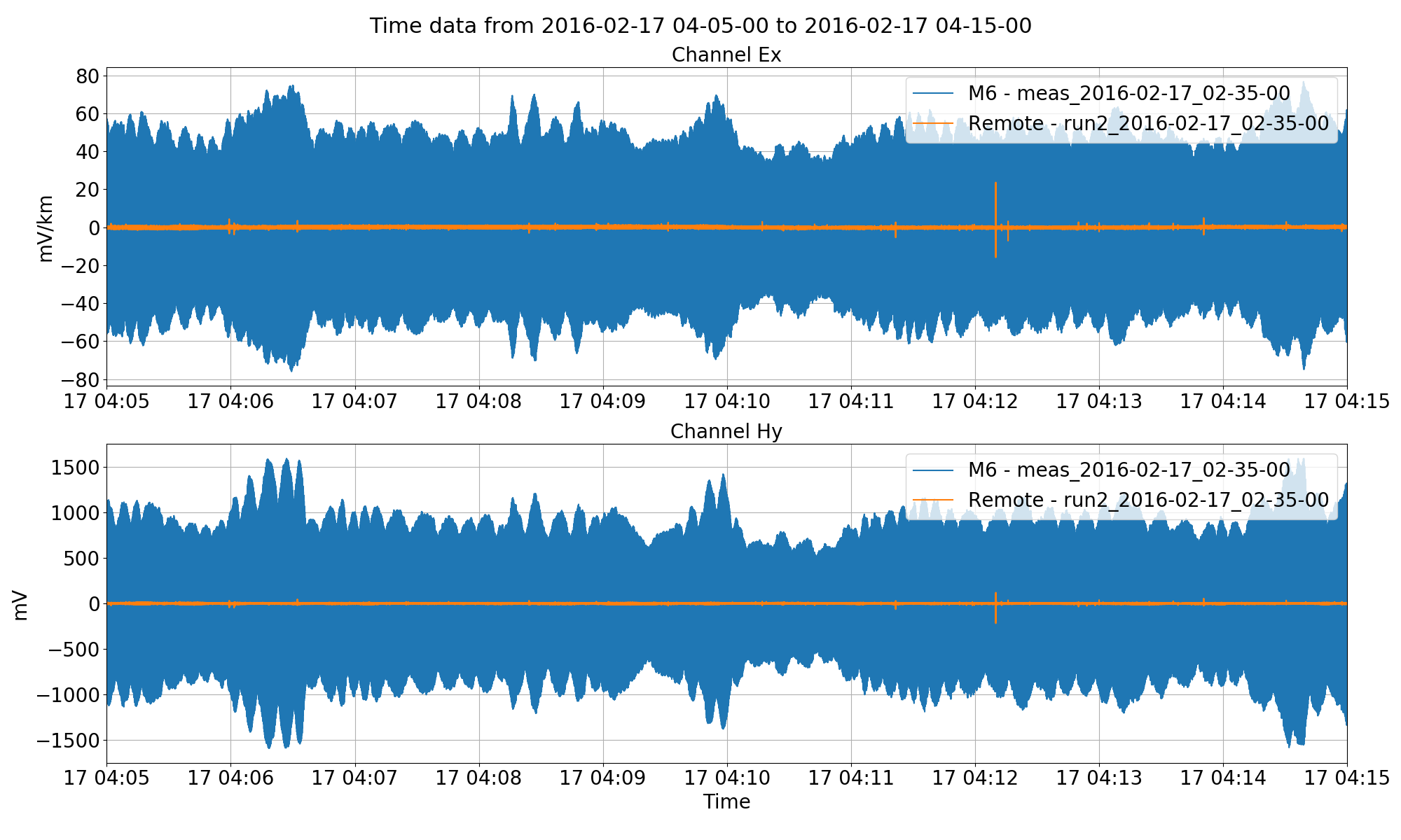
Site M6 vs. Remote unfiltered. Site M6 is much noisier and has significant high amplitude powerline noise consistent with a developed area.
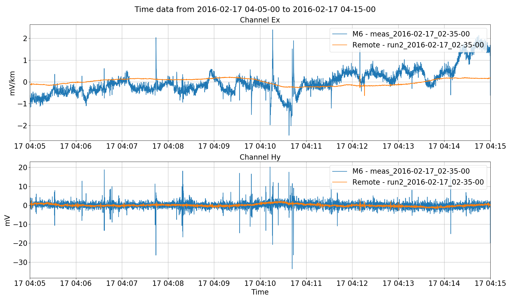
Site M6 vs. Remote filtered to 4 Hz. The longer period data is easier to see here, though M6 still has much more noise in the recordings.
Single site impedance tensor
The next step is to process the data, in the first instance using simple single site processing. Single site processing should be familiar from the Tutorial and begins with calculating the spectra and continues with calculating the magnetotellruic transfer function and plotting the impedance tensor.
1 2 3 4 5 6 7 8 9 10 11 12 13 14 15 16 17 18 19 20 21 22 23 24 25 26 27 28 29 30 31 32 33 34 35 36 | from datapaths import remotePath, remoteImages
from resistics.project.io import loadProject
from resistics.project.spectra import calculateSpectra
from resistics.project.transfunc import processProject, viewImpedance
from resistics.project.statistics import calculateStatistics, viewStatistic
from resistics.project.mask import newMaskData, calculateMask
from resistics.common.plot import plotOptionsTransferFunction, getPaperFonts
plotOptions = plotOptionsTransferFunction(plotfonts=getPaperFonts())
proj = loadProject(remotePath)
# calculate spectrum using standard options
calculateSpectra(proj, sites=["M6", "Remote"])
proj.refresh()
# single site processing
processProject(proj, sites=["M6", "Remote"])
# 128 Hz impedance tensor estimates
figs = viewImpedance(
proj,
sites=["M6", "Remote"],
sampleFreqs=[128],
oneplot=False,
plotoptions=plotOptions,
show=False,
save=False,
)
figs[0].savefig(remoteImages / "singleSiteM6_128.png")
figs[1].savefig(remoteImages / "singleSiteRemote_128.png")
# all sampling frequencies for M6
figs = viewImpedance(
proj, sites=["M6"], oneplot=False, plotoptions=plotOptions, show=False, save=False
)
figs[0].savefig(remoteImages / "singleSiteM6_all.png")
|
As the higher frequencies of Site M6 have also been processed, these can be plotted with the 128 Hz to give more periods.
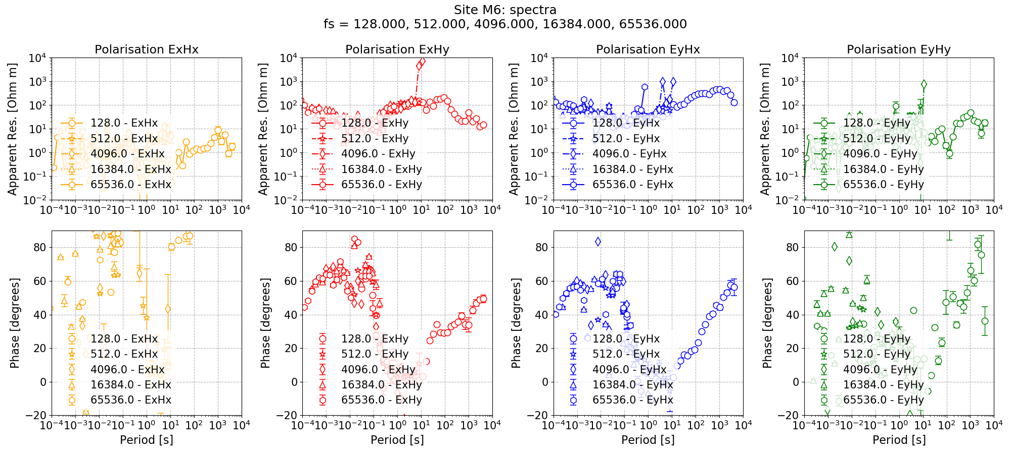
Impedance tensor estimates for Site M6 at all frequencies
Howver, of more interest for this example is the impedance tensor estimates using data sampled at 128 Hz, the sampling frequency at which remote reference processing will be used. The single site impedance tensor estimates for 128 Hz are given below.
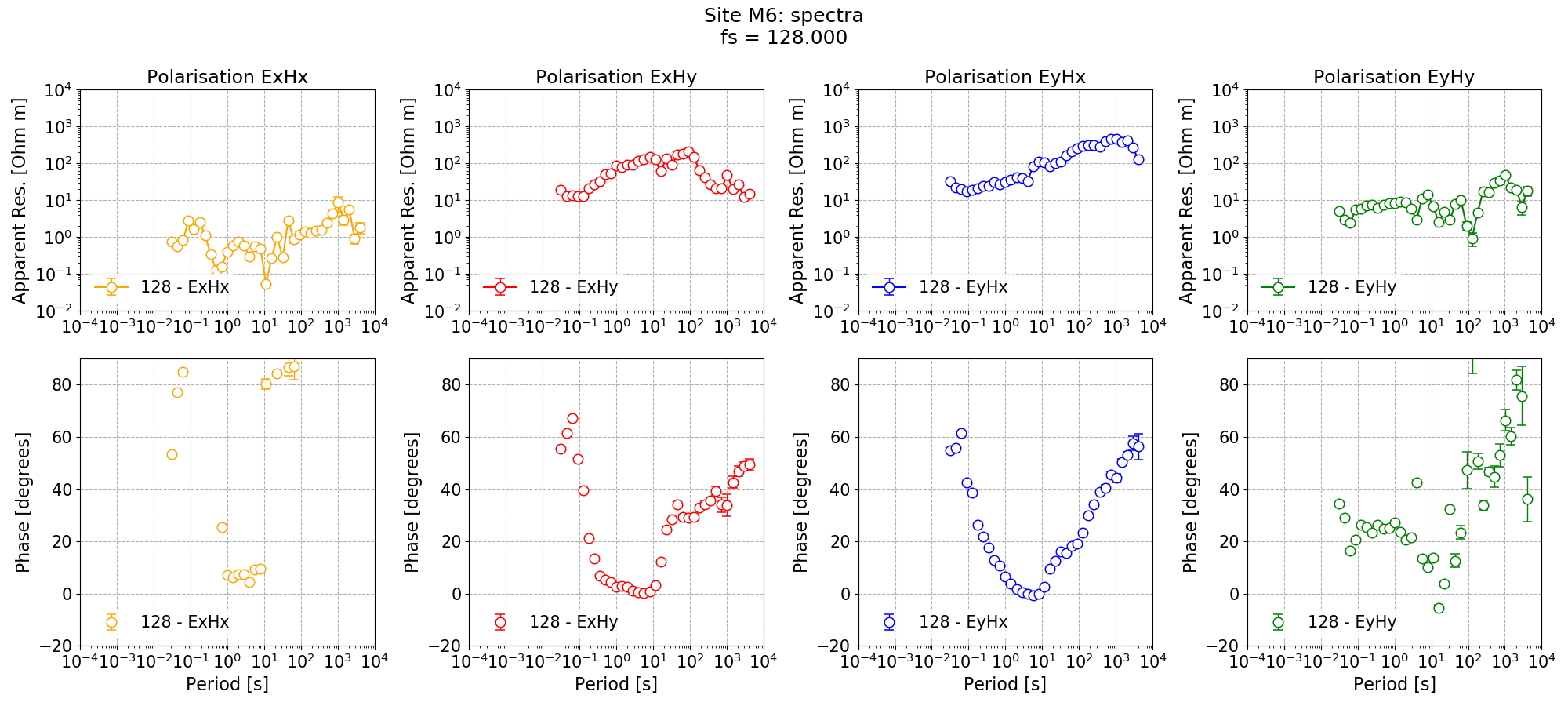
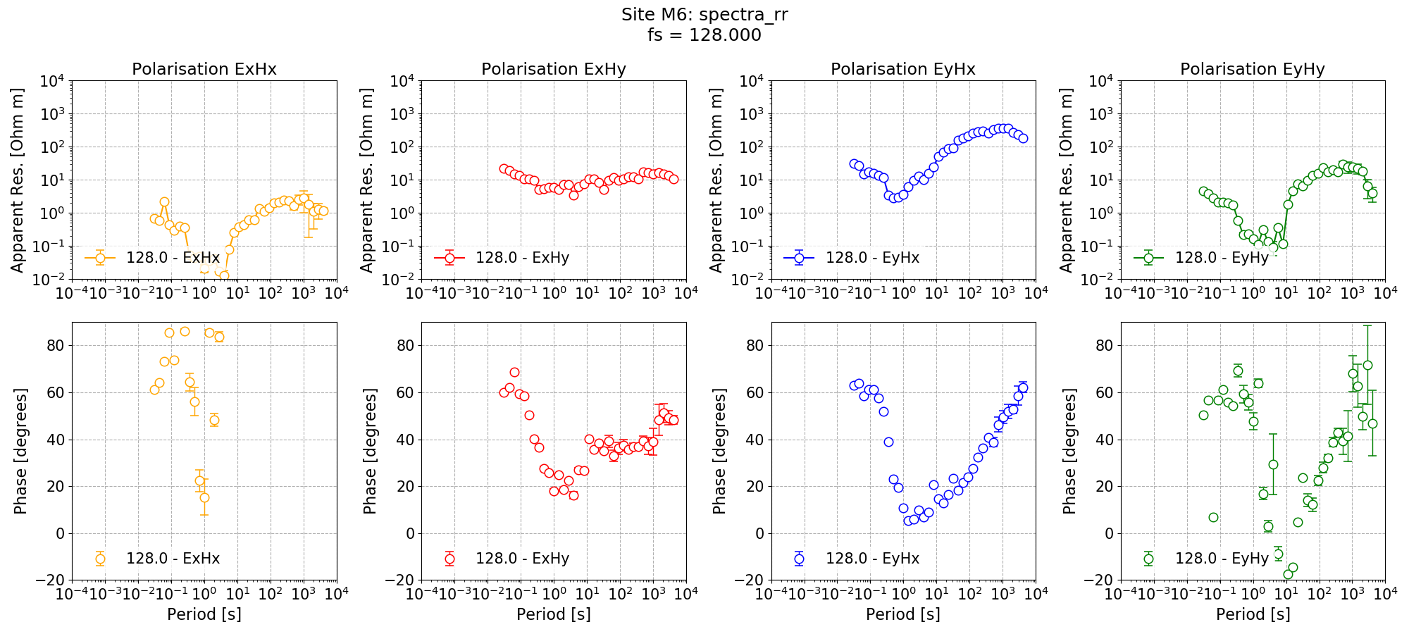
Single site impedance tensor estimates for Site M6 at 128 Hz
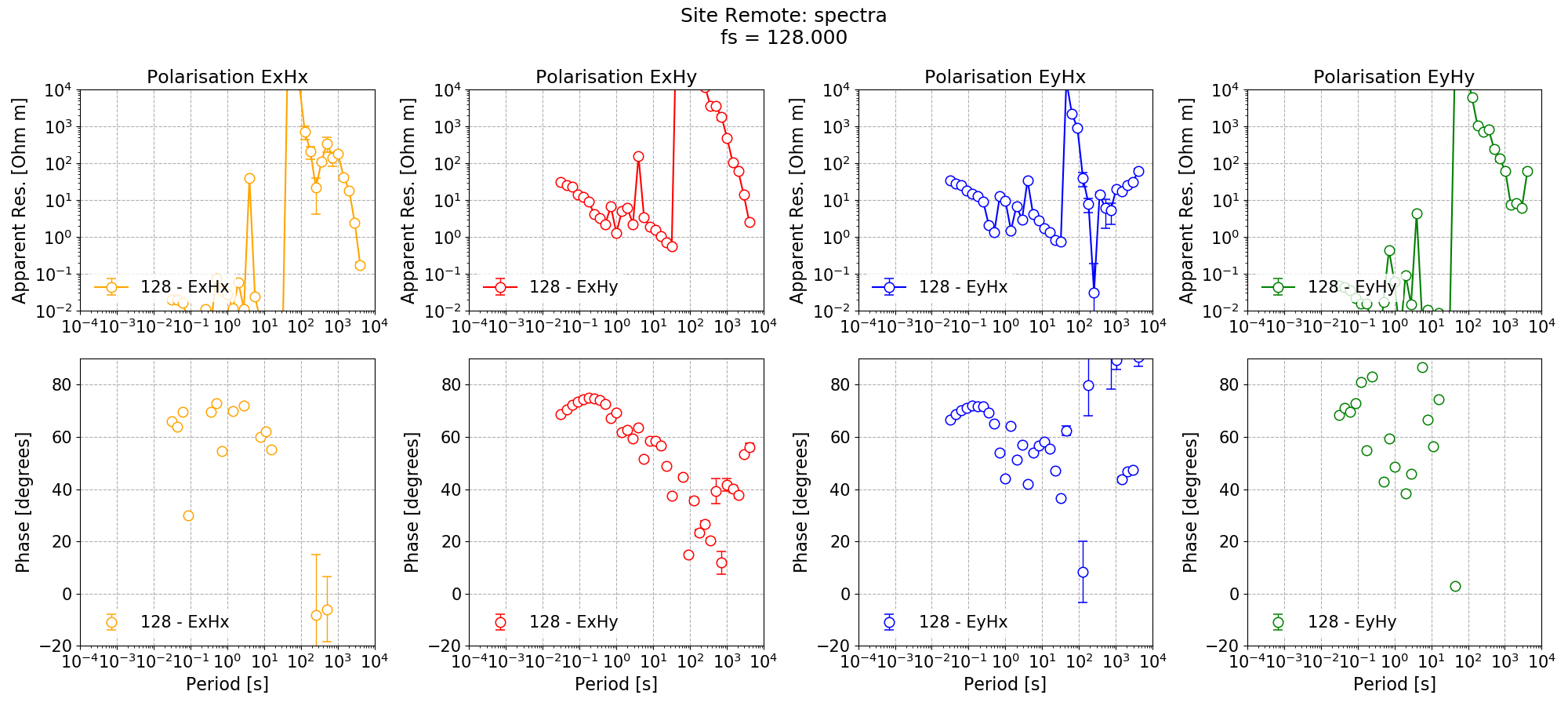
Single site impedance tensor estimates for the Remote site at 128 Hz
Neither of the estimates are great. Site Remote looks poor and noisy. Site M6 appears to be biased in the dead band with the phase going to near 0. However, for the time being, continue to perform standard remote reference processing.
Remote reference impedance tensor
Standard remote reference processing is performed using the processProject() method of module transfunc.
38 39 40 41 42 43 44 45 46 47 48 49 50 51 | # perform standard remote reference runs - remember to call the output something else
processProject(
proj, sites=["M6"], sampleFreqs=[128], remotesite="Remote", postpend="rr"
)
figs = viewImpedance(
proj,
sites=["M6"],
postpend="rr",
oneplot=False,
plotoptions=plotOptions,
show=False,
save=False,
)
figs[0].savefig(remoteImages / "remoteReferenceM6.png")
|
To perform remote reference processing, the sites to process have been defined using the sites = [“M6”] keyword argument. Further, a remote site has been defined using the remotesite = “Remote” keyword argument. Specifying a remote site will ensure remote reference processing of data which overlaps in time between the sites and the remote site.
Again, the impedance tensor has been plotted and the plot is provided below.
Standard remote reference impedance tensor estimate for Site M6.
Single site statistics
As a next step, calculate single site statistics separately for M6 and Remote, produce a simple coherence mask with a threshold of 0.8 and redo the single site processing. For more information about statistics, please see the tutorial and statistics.
53 54 55 56 57 58 59 60 61 62 63 64 65 66 67 68 69 70 71 72 73 74 75 76 77 78 79 80 81 82 83 84 85 | # let's calculate some single site statistics
calculateStatistics(proj, sites=["M6", "Remote"], stats=["coherence", "transferFunction"])
# calculate masks
maskData = newMaskData(proj, 128)
maskData.setStats(["coherence"])
maskData.addConstraint("coherence", {"cohExHy": [0.8, 1.0], "cohEyHx": [0.8, 1.0]})
maskData.maskName = "coh80_100"
maskData.printInfo()
maskData.printConstraints()
# calculate
calculateMask(proj, maskData, sites=["M6", "Remote"])
# single site processing again
processProject(
proj,
sites=["M6", "Remote"],
sampleFreqs=[128],
masks={"M6": "coh80_100", "Remote": "coh80_100"},
postpend="coh80_100",
)
figs = viewImpedance(
proj,
sites=["M6", "Remote"],
sampleFreqs=[128],
postpend="coh80_100",
oneplot=False,
plotoptions=plotOptions,
show=False,
save=False,
)
figs[0].savefig(remoteImages / "singleSiteM6_128_coh80.png")
figs[1].savefig(remoteImages / "singleSiteRemote_128_coh80.png")
|
The single site impedance tensors processed with the masks are shown below.
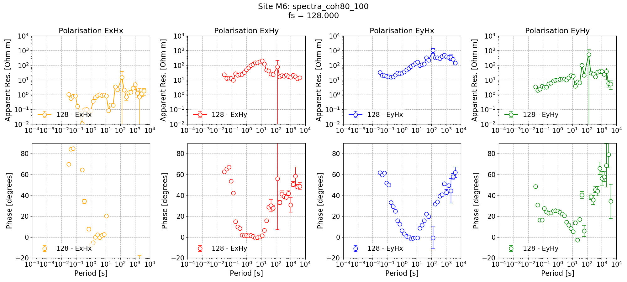
Single site impedance tensor estimates for Site M6 at 128 Hz using a coherency mask excluding windows with coherence Ex-Hy or Ey-Hx below 0.8.
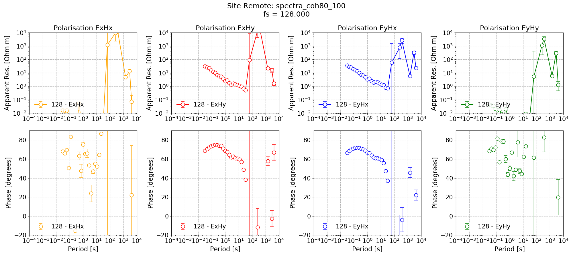
Single site impedance tensor estimates for the Remote site at 128 Hz using a coherency mask excluding windows with coherence Ex-Hy or Ey-Hx below 0.8.
Coherence masking has done little to improve the impedance tensor estimates for Site M6. However, it has noticeably improved the estimate for Remote. With this in mind, the next step is to do remote reference processing, but excluding windows where Remote site has Ex-Hy or Ey-Hx coherency below 0.8. This is done as follows:
87 88 89 90 91 92 93 94 95 96 97 98 99 100 101 102 103 104 105 106 107 | # remote reference processing with masks
processProject(
proj,
sites=["M6"],
sampleFreqs=[128],
remotesite="Remote",
masks={"Remote": "coh80_100"},
postpend="rr_coh80_100",
)
figs = viewImpedance(
proj,
sites=["M6"],
sampleFreqs=[128],
postpend="rr_coh80_100",
oneplot=False,
plotoptions=plotOptions,
show=False,
save=False,
)
figs[0].savefig(remoteImages / "remoteReferenceM6_128_coh80.png")
|
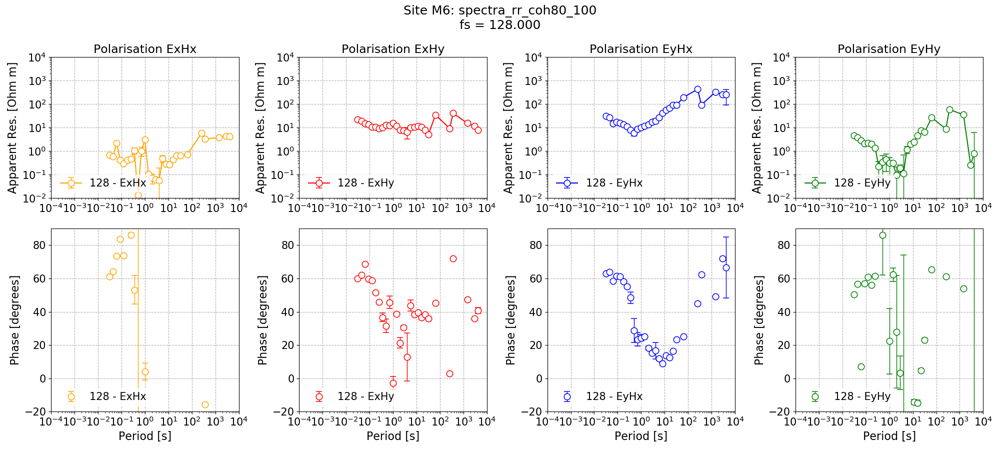
Remote reference impedance tensor estimates for Site M6 at 128 Hz using a coherency mask on the Remote data excluding windows with coherence Ex-Hy or Ey-Hx below 0.8.
The resultant remote reference impedance tensor estimate for Site M6 has improved in some places, mainly in the Ey-Hx polarisation. However, after a period of 102 seconds, the results are poor. This matches the single site impedance tensor for Remote after 102 seconds, where the results are equally incorrect, possibly because of too few windows.
Date and time constraints
Finally, another way to restrict the data being used for remote reference processing is to use datetime restrictions. Datetime restrictions were introduced in the tutorial and datetime constraints.
109 110 111 112 113 114 115 116 117 118 119 120 121 122 123 124 125 126 127 128 129 | # remote reference processing with datetime constraints
processProject(
proj,
sites=["M6"],
sampleFreqs=[128],
remotesite="Remote",
datetimes=[{"type": "time", "start": "20:00:00", "stop": "07:00:00"}],
postpend="rr_night",
)
figs = viewImpedance(
proj,
sites=["M6"],
sampleFreqs=[128],
postpend="rr_night",
oneplot=False,
plotoptions=plotOptions,
show=False,
save=False,
)
figs[0].savefig(remoteImages / "remoteReferenceM6_128_coh80_datetimes.png")
|
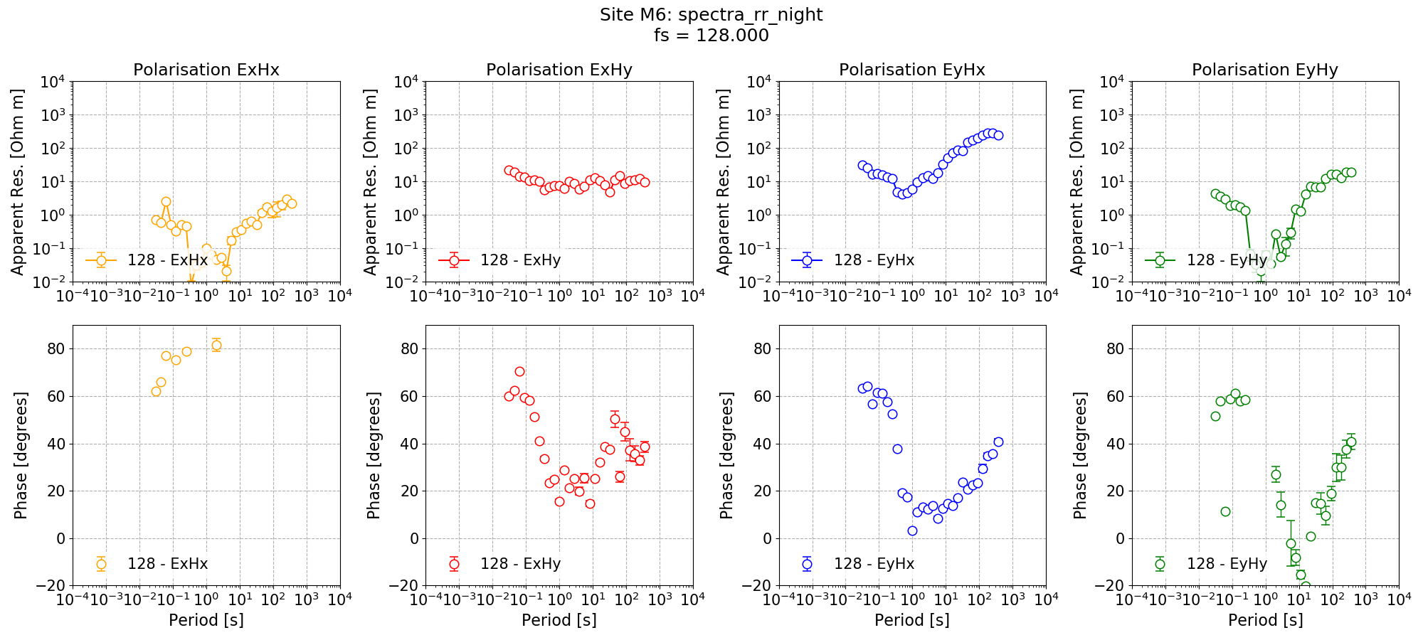
Remote reference impedance tensor estimates of Site M6 with datetime constraints using only night time data.
In the next section, remote reference statistics will be introduced. These are different to single site statistics in that they combine data from the local site and remote reference site.
Complete example scripts
For the purposes of clarity, the complete example scripts are provided below.
For pre-processing:
1 2 3 4 5 6 7 8 9 10 11 12 13 14 15 16 17 18 19 20 21 22 23 24 25 26 27 28 29 30 31 32 33 34 35 36 37 38 39 40 41 42 43 44 45 46 47 48 49 50 51 52 53 54 55 56 57 58 59 60 61 62 | from datapaths import remotePath, remoteImages
from resistics.project.io import loadProject
from resistics.project.time import preProcess, viewTime
proj = loadProject(remotePath)
proj.printInfo()
# get information about the local site
siteLocal = proj.getSiteData("M6")
siteLocal.printInfo()
# get information about the SPAM data remote reference
siteRemote = proj.getSiteData("RemoteSPAM")
siteRemote.printInfo()
# want to resample the RemoteSPAM data to 128 Hz
# SPAM data want to resample onto the second
# to make sure the times are matching, we can loop through the 128Hz measurements of M6 and use those times
meas128 = siteLocal.getMeasurements(128)
for meas in meas128:
    start = siteLocal.getMeasurementStart(meas).strftime("%Y-%m-%d %H:%M:%S")
    stop = siteLocal.getMeasurementEnd(meas).strftime("%Y-%m-%d %H:%M:%S")
    postpend = siteLocal.getMeasurementStart(meas).strftime("%Y-%m-%d_%H-%M-%S")
    print("Processing data from {} to {}".format(start, stop))
    preProcess(
        proj,
        sites="RemoteSPAM",
        start=start,
        stop=stop,
        interp=True,
        resamp={250: 128},
        outputsite="Remote",
        prepend="",
        postpend=postpend,
    )
proj.refresh()
from resistics.common.plot import plotOptionsTime, getPresentationFonts
plotOptions = plotOptionsTime(plotfonts=getPresentationFonts())
fig = viewTime(
proj,
sites=["M6", "Remote"],
startDate="2016-02-17 04:05:00",
endDate="2016-02-17 04:15:00",
chans=["Ex", "Hy"],
plotoptions=plotOptions,
save=False,
show=False,
)
fig.savefig(remoteImages / "viewTimePreprocess.png")
fig = viewTime(
proj,
sites=["M6", "Remote"],
startDate="2016-02-17 04:05:00",
endDate="2016-02-17 04:15:00",
filter={"lpfilt": 4},
chans=["Ex", "Hy"],
plotoptions=plotOptions,
save=False,
show=False,
)
fig.savefig(remoteImages / "viewTimePreprocessLowPass.png")
|
For estimating imepdance tensors:
1 2 3 4 5 6 7 8 9 10 11 12 13 14 15 16 17 18 19 20 21 22 23 24 25 26 27 28 29 30 31 32 33 34 35 36 37 38 39 40 41 42 43 44 45 46 47 48 49 50 51 52 53 54 55 56 57 58 59 60 61 62 63 64 65 66 67 68 69 70 71 72 73 74 75 76 77 78 79 80 81 82 83 84 85 86 87 88 89 90 91 92 93 94 95 96 97 98 99 100 101 102 103 104 105 106 107 108 109 110 111 112 113 114 115 116 117 118 119 120 121 122 123 124 125 126 127 128 129 | from datapaths import remotePath, remoteImages
from resistics.project.io import loadProject
from resistics.project.spectra import calculateSpectra
from resistics.project.transfunc import processProject, viewImpedance
from resistics.project.statistics import calculateStatistics, viewStatistic
from resistics.project.mask import newMaskData, calculateMask
from resistics.common.plot import plotOptionsTransferFunction, getPaperFonts
plotOptions = plotOptionsTransferFunction(plotfonts=getPaperFonts())
proj = loadProject(remotePath)
# calculate spectrum using standard options
calculateSpectra(proj, sites=["M6", "Remote"])
proj.refresh()
# single site processing
processProject(proj, sites=["M6", "Remote"])
# 128 Hz impedance tensor estimates
figs = viewImpedance(
proj,
sites=["M6", "Remote"],
sampleFreqs=[128],
oneplot=False,
plotoptions=plotOptions,
show=False,
save=False,
)
figs[0].savefig(remoteImages / "singleSiteM6_128.png")
figs[1].savefig(remoteImages / "singleSiteRemote_128.png")
# all sampling frequencies for M6
figs = viewImpedance(
proj, sites=["M6"], oneplot=False, plotoptions=plotOptions, show=False, save=False
)
figs[0].savefig(remoteImages / "singleSiteM6_all.png")
# perform standard remote reference runs - remember to call the output something else
processProject(
    proj, sites=["M6"], sampleFreqs=[128], remotesite="Remote", postpend="rr"
)
figs = viewImpedance(
    proj,
    sites=["M6"],
    postpend="rr",
    oneplot=False,
    plotoptions=plotOptions,
    show=False,
    save=False,
)
figs[0].savefig(remoteImages / "remoteReferenceM6.png")
# let's calculate some single site statistics
calculateStatistics(proj, sites=["M6", "Remote"], stats=["coherence", "transferFunction"])

# calculate masks
maskData = newMaskData(proj, 128)
maskData.setStats(["coherence"])
maskData.addConstraint("coherence", {"cohExHy": [0.8, 1.0], "cohEyHx": [0.8, 1.0]})
maskData.maskName = "coh80_100"
maskData.printInfo()
maskData.printConstraints()
# calculate
calculateMask(proj, maskData, sites=["M6", "Remote"])

# single site processing again
processProject(
    proj,
    sites=["M6", "Remote"],
    sampleFreqs=[128],
    masks={"M6": "coh80_100", "Remote": "coh80_100"},
    postpend="coh80_100",
)
figs = viewImpedance(
    proj,
    sites=["M6", "Remote"],
    sampleFreqs=[128],
    postpend="coh80_100",
    oneplot=False,
    plotoptions=plotOptions,
    show=False,
    save=False,
)
figs[0].savefig(remoteImages / "singleSiteM6_128_coh80.png")
figs[1].savefig(remoteImages / "singleSiteRemote_128_coh80.png")
# remote reference processing with masks
processProject(
    proj,
    sites=["M6"],
    sampleFreqs=[128],
    remotesite="Remote",
    masks={"Remote": "coh80_100"},
    postpend="rr_coh80_100",
)

figs = viewImpedance(
    proj,
    sites=["M6"],
    sampleFreqs=[128],
    postpend="rr_coh80_100",
    oneplot=False,
    plotoptions=plotOptions,
    show=False,
    save=False,
)
figs[0].savefig(remoteImages / "remoteReferenceM6_128_coh80.png")
# remote reference processing with datetime constraints
processProject(
    proj,
    sites=["M6"],
    sampleFreqs=[128],
    remotesite="Remote",
    datetimes=[{"type": "time", "start": "20:00:00", "stop": "07:00:00"}],
    postpend="rr_night",
)

figs = viewImpedance(
    proj,
    sites=["M6"],
    sampleFreqs=[128],
    postpend="rr_night",
    oneplot=False,
    plotoptions=plotOptions,
    show=False,
    save=False,
)
figs[0].savefig(remoteImages / "remoteReferenceM6_128_coh80_datetimes.png")
|