Remote reference with configuration
Slowly, the remote reference result of Site M6 has been improving, but there are still some issues:
The long period
The dead band
The dead band is a challenging issue in magnetotellurics due to the poor signal-to-noise ratio. However, one thing that can be done to improve the long period is to change the minimum window size so there are more windows at high decimation levels (long periods).
Simple configuration
Configuration files provide an easy way to define processing parameters. They are described in more detail here and here.
The below configuration file changes the decimation scheme to 8 decimation levels with 5 evaluation frequencies per level and the minimum window size. In addition, the remote statistics to calculate have been explicitly defined so they do not need to be specifed in the call to calculateRemoteStatistics().
1 2 3 4 5 6 7 8 9 10 11 12 13 14 15 16 17 | name = dec8_5
[Spectra]
specdir = "dec8_5"
[Decimation]
numlevels = 8
[Frequencies]
perlevel = 5
[Window]
minwindowsize = 256
minoverlapsize = 64
[Statistics]
remotestats = "RR_coherenceEqn",
|
As the decimation parameters have changed, the spectra need to be recalculated. The specdir option has also been changed, meaning that the spectra will be saved in a different directory and avoiding any future issues.
Important
It is important to understand the specdir (spectra directory) options in resistics to avoid future problems. For more information, please read Multiple Spectra.
The following recalculates the spectra, the single site impedance tensors, the remote reference statistics, the mask and the remote reference impedance tensor.
1 2 3 4 5 6 7 8 9 10 11 12 13 14 15 16 17 18 19 20 21 22 23 24 25 26 27 28 29 30 31 32 33 34 35 36 37 38 39 40 41 42 43 44 45 46 47 48 49 50 51 52 53 54 55 56 57 58 59 60 61 62 63 64 65 66 67 | from datapaths import remotePath, remoteImages
from resistics.project.io import loadProject
from resistics.project.spectra import calculateSpectra
from resistics.project.transfunc import processProject, viewImpedance
from resistics.project.statistics import calculateRemoteStatistics, viewStatistic
from resistics.project.mask import newMaskData, calculateMask
from resistics.common.plot import plotOptionsTransferFunction, getPaperFonts
plotOptions = plotOptionsTransferFunction(plotfonts=getPaperFonts())
proj = loadProject(remotePath, "remoteConfig.ini")
calculateSpectra(proj, sites=["M6", "Remote"])
proj.refresh()
# single site processing
processProject(proj, sites=["M6", "Remote"])
figs = viewImpedance(
proj,
sites=["M6", "Remote"],
sampleFreqs=[128],
oneplot=False,
plotoptions=plotOptions,
save=False,
show=False,
)
figs[0].savefig(remoteImages / "singleSiteM6_128_dec8_5.png")
figs[1].savefig(remoteImages / "singleSiteRemote_128_dec8_5.png")
# calculate the statistic we are interested in
calculateRemoteStatistics(proj, "Remote", sites=["M6"], sampleFreqs=[128])
# generate mask
maskData = newMaskData(proj, 128)
maskData.setStats(["RR_coherenceEqn"])
maskData.addConstraint(
"RR_coherenceEqn", {"ExHyR-HyHyR": [0.8, 1.0], "EyHxR-HxHxR": [0.8, 1.0]}
)
# finally, lets give maskData a name, which will relate to the output file
maskData.maskName = "rr_cohEqn_80_100"
calculateMask(proj, maskData, sites=["M6"])
maskData.printInfo()
# process with masks
processProject(
proj,
sites=["M6"],
sampleFreqs=[128],
remotesite="Remote",
masks={"M6": "rr_cohEqn_80_100"},
datetimes=[
{"type": "time", "start": "20:00:00", "stop": "07:00:00", "levels": [0, 1]}
],
postpend="rr_cohEqn_80_100_night",
)
figs = viewImpedance(
proj,
sites=["M6"],
sampleFreqs=[128],
postpend="rr_cohEqn_80_100_night",
oneplot=False,
plotoptions=plotOptions,
save=False,
show=False,
)
figs[0].savefig(remoteImages / "remoteReferenceM6_128_RR_dec8_5_coh_datetime_01.png")
|
The single site impedance tensor estimates are shown below.
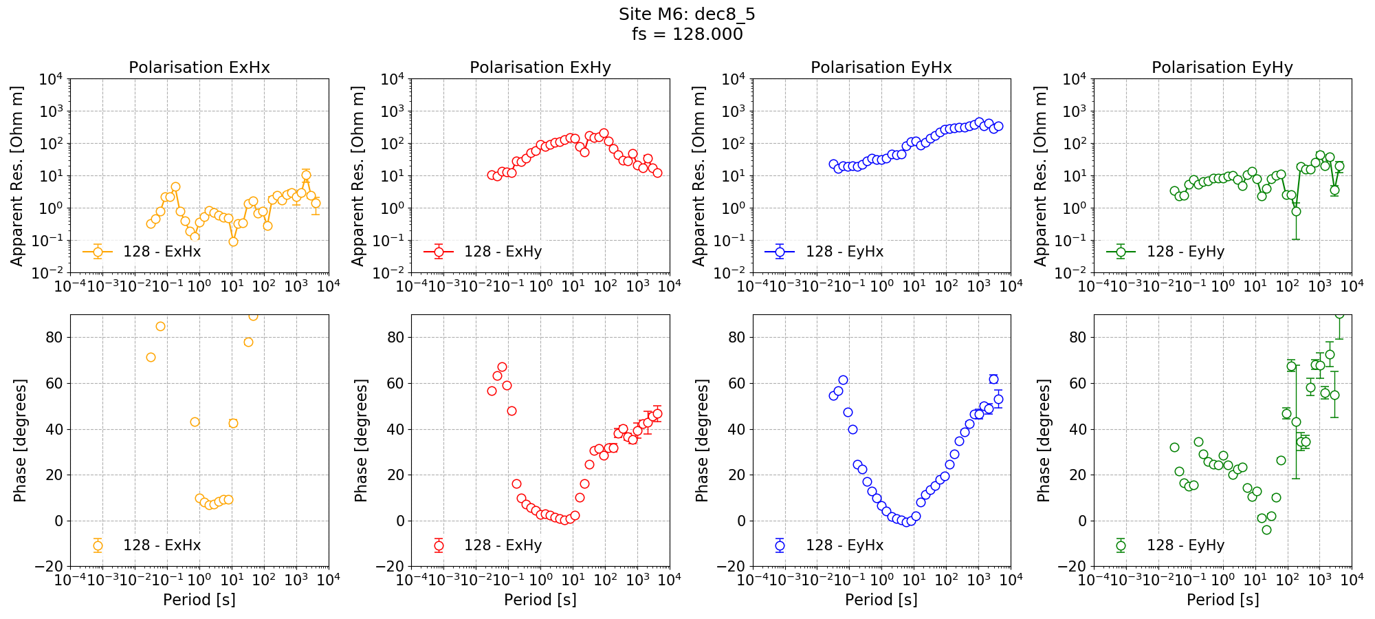
Single site impedance tensor estimates for Site M6 at 128 Hz using 8 decimation levels and 5 evaluation frequencies per level with a minimum window size of 256 points.

Single site impedance tensor estimates for the Remote site at 128 Hz using 8 decimation levels and 5 evaluation frequencies per level with a minimum window size of 256 points.
The long periods have now improved, particularly for the Remote site. However, the dead band remains an issue for Remote and Site M6.
The remote reference processing result for Site M6 is shown below. The long periods are noticeably better in both phase and apparent resistivity than the results with the standard processing scheme. As stated earlier, the dead band shows no discernible improvement.

Remote reference impedance tensor estimates for Site M6 at 128 Hz using 8 decimation levels and 5 evaluation frequencies per level with a minimum window size of 256 points. Masks and time constraints are applied.
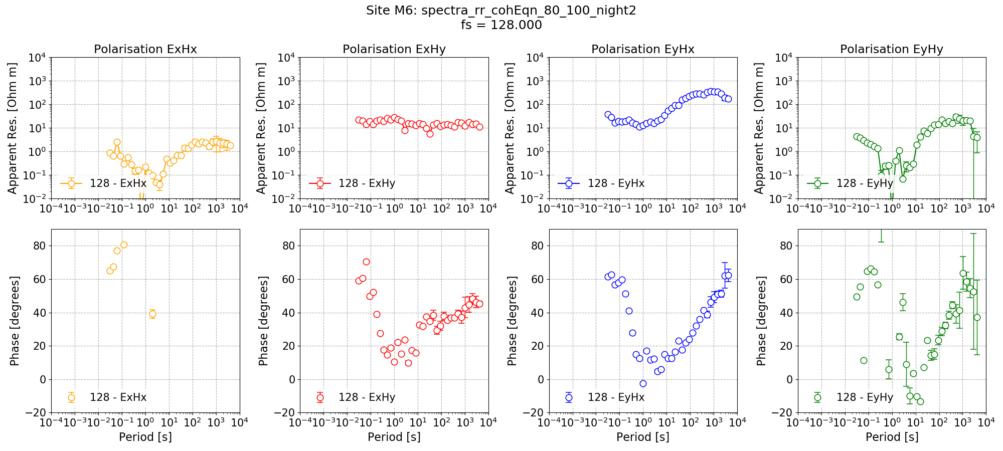
Remote reference impedance tensor estimates for Site M6 at 128 Hz using the standard decimation and evaluation scheme. The same masks and time constraints are applied.
Customised windowing
Resistics gives fine grained control over windowing and overlaps. In the below configuration file, the same decimation scheme is used, with 8 decimation levels and 5 evaluation frequencies per level. However, the windowing has been defined explicitly for each decimation level. In addition and similar to the dec8_5 configuration file, the statistics and remote statistics to calculate have been explicitly defined so they do not need to be specifed in calls to calculateStatistics() and calculateRemoteStatistics().
1 2 3 4 5 6 7 8 9 10 11 12 13 14 15 16 17 18 | name = man8_5
[Spectra]
specdir = "man8_5"
[Decimation]
numlevels = 8
[Frequencies]
perlevel = 5
[Window]
windowsizes = 1024, 512, 512, 256, 256, 256, 256, 256
overlapsizes = 256, 128, 128, 64, 64, 64, 64, 64
[Statistics]
stats = "coherence",
remotestats = "RR_coherenceEqn",
|
Like with the dec8_5 configuration file, begin with single site processing.
1 2 3 4 5 6 7 8 9 10 11 12 13 14 15 16 17 18 19 20 21 22 23 24 25 26 27 28 29 30 31 32 33 34 35 36 37 38 39 40 41 42 43 44 45 46 47 48 49 50 51 52 53 54 55 56 57 58 59 60 61 62 63 | from datapaths import remotePath, remoteImages
from resistics.project.io import loadProject
from resistics.project.spectra import calculateSpectra
from resistics.project.transfunc import processProject, viewImpedance
from resistics.project.statistics import (
calculateStatistics,
calculateRemoteStatistics,
viewStatistic,
)
from resistics.project.mask import newMaskData, calculateMask
from resistics.common.plot import plotOptionsTransferFunction, getPaperFonts
plotOptions = plotOptionsTransferFunction(plotfonts=getPaperFonts())
proj = loadProject(remotePath, "manualWindowsConfig.ini")
# calculate spectra
calculateSpectra(proj, sites=["M6", "Remote"])
proj.refresh()
processProject(proj, sites=["M6", "Remote"])
figs = viewImpedance(
proj,
sites=["M6", "Remote"],
sampleFreqs=[128],
oneplot=False,
plotoptions=plotOptions,
save=False,
show=False,
)
figs[0].savefig(remoteImages / "singleSiteM6_128_man8_5.png")
figs[1].savefig(remoteImages / "singleSiteRemote_128_man8_5.png")
# calculate the statistic we are interested in
calculateStatistics(proj, sites=["M6", "Remote"], sampleFreqs=[128])
calculateRemoteStatistics(proj, "Remote", sites=["M6"], sampleFreqs=[128])
# generate single site masks
maskData = newMaskData(proj, 128)
maskData.setStats(["coherence"])
maskData.addConstraint("coherence", {"cohExHy": [0.8, 1.0], "cohEyHx": [0.8, 1.0]})
# finally, lets give maskData a name, which will relate to the output file
maskData.maskName = "coh_80_100"
calculateMask(proj, maskData, sites=["M6", "Remote"])
maskData.printInfo()
# process remote on its own to compare to the first processing we did
processProject(
proj,
sites=["Remote"],
sampleFreqs=[128],
masks={"Remote": "coh_80_100"},
postpend="coh_80_100",
)
figs = viewImpedance(
proj,
sites=["Remote"],
sampleFreqs=[128],
postpend="coh_80_100",
oneplot=False,
plotoptions=plotOptions,
save=False,
show=False,
)
figs[0].savefig(remoteImages / "singleSiteRemote_128_man8_5_coh80.png")
|

Single site impedance tensor estimates for Site M6 at 128 Hz using 8 decimation levels and 5 evaluation frequencies per level with a custom window size per decimation level.
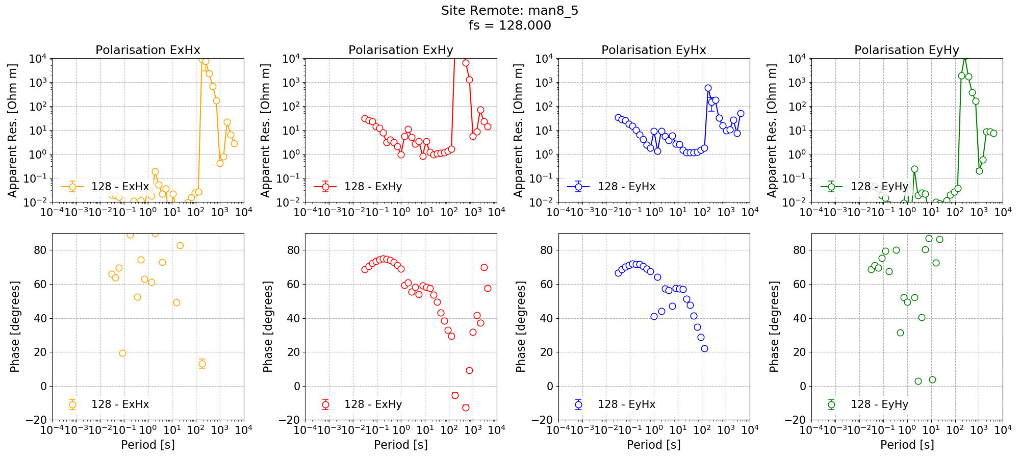
Single site impedance tensor estimates for the Remote site at 128 Hz using 8 decimation levels and 5 evaluation frequencies per level with a custom window size per decimation level.
In addition to single site processing, Remote is processed with a coherence mask giving the below impedance tensor estimate.
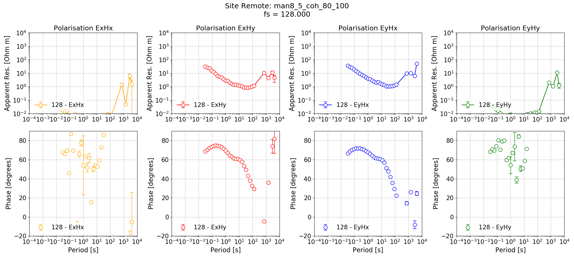
Single site impedance tensor estimates for the Remote site at 128 Hz using 8 decimation levels and 5 evaluation frequencies per level with a custom window size per decimation level. A coherence mask of 0.8 has applied to discard noisy windows.
Applying the coherence mask has significantly improved the single site impedance tensor estimates for Remote in the dead band. However, in some cases, it has left no windows at the long periods (this is clear from the missing markers for some evaluation frequencies).
Next, the same remote reference processing is repeated with matching parameters to the dec8_5 processing as shown below.
65 66 67 68 69 70 71 72 73 74 75 76 77 78 79 80 81 82 83 84 85 86 87 88 89 90 91 92 93 94 95 96 97 98 | # generate mask
maskData = newMaskData(proj, 128)
maskData.setStats(["RR_coherenceEqn"])
maskData.addConstraint(
"RR_coherenceEqn", {"ExHyR-HyHyR": [0.8, 1.0], "EyHxR-HxHxR": [0.8, 1.0]}
)
# finally, lets give maskData a name, which will relate to the output file
maskData.maskName = "rr_cohEqn_80_100"
calculateMask(proj, maskData, sites=["M6"])
maskData.printInfo()
# process with masks
processProject(
proj,
sites=["M6"],
sampleFreqs=[128],
remotesite="Remote",
masks={"M6": "rr_cohEqn_80_100"},
datetimes=[
{"type": "time", "start": "20:00:00", "stop": "07:00:00", "levels": [0, 1]}
],
postpend="rr_cohEqn_80_100_night",
)
figs = viewImpedance(
proj,
sites=["M6"],
sampleFreqs=[128],
postpend="rr_cohEqn_80_100_night",
oneplot=False,
plotoptions=plotOptions,
save=False,
show=False,
)
figs[0].savefig(remoteImages / "remoteReferenceM6_128_RR_man8_5_coh_datetime_01.png")
|
The resultant remote reference impedance tensor estimate for Site M6 is shown below.
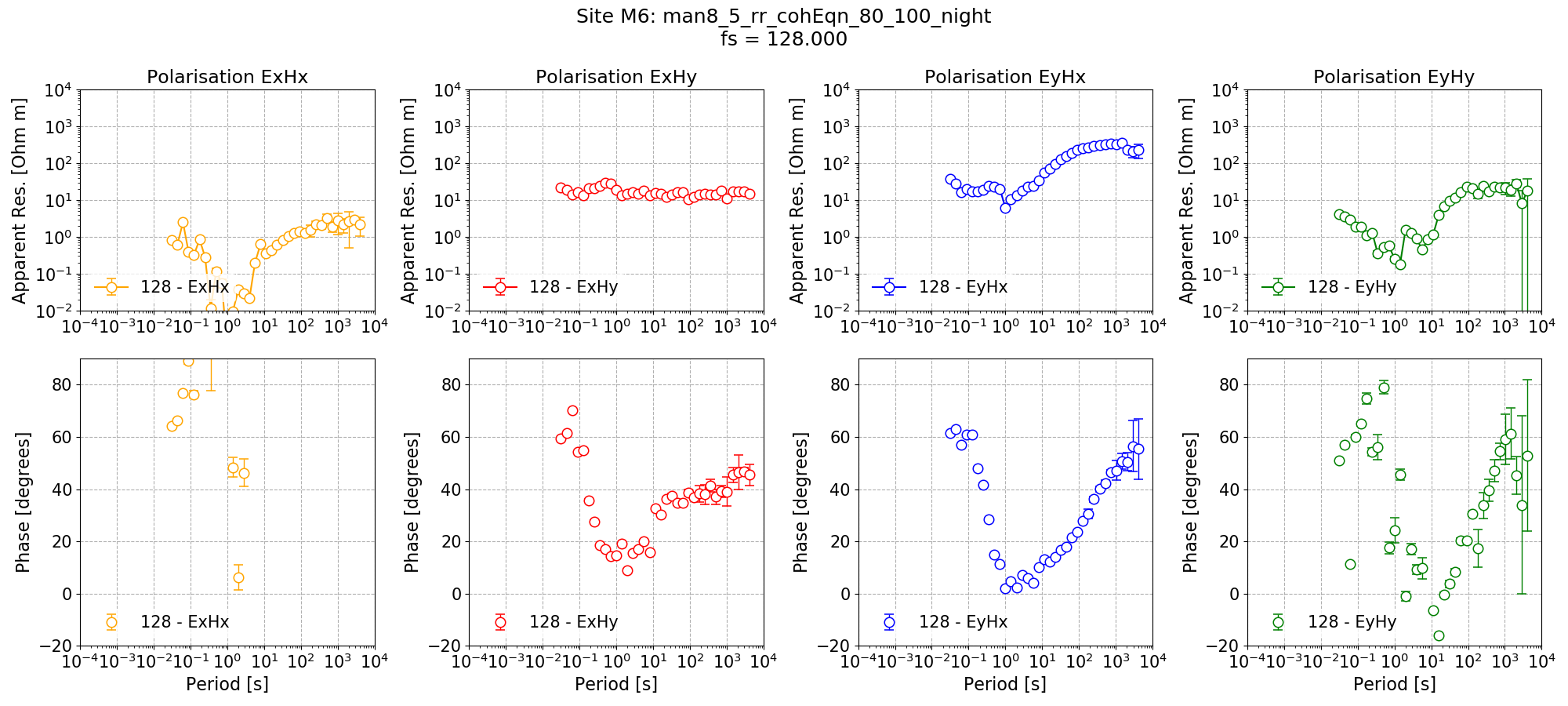
Remote reference impedance tensor estimates for Site M6 at 128 Hz using 8 decimation levels and 5 evaluation frequencies per level with a custom window size per decimation level. Masks and time constraints are applied.
In general, the results are comparable with the other decimation/windowing schemes and are better in some places such as the long periods, and similar in others.
As an additional test, another mask is applied, which is the single site mask for Remote excluding Remote windows with coherence Ex-Hy or Ey-Hx below 0.8.
100 101 102 103 104 105 106 107 108 109 110 111 112 113 114 115 116 117 118 119 120 121 122 123 | # one more example with multiple masks
# let's use standard coherence as well for Remote only
processProject(
proj,
sites=["M6"],
sampleFreqs=[128],
remotesite="Remote",
masks={"M6": ["rr_cohEqn_80_100"], "Remote": "coh_80_100"},
datetimes=[
{"type": "time", "start": "20:00:00", "stop": "07:00:00", "levels": [0, 1]}
],
postpend="rr_cohEqn_80_100_and_coh_80_100_night",
)
figs = viewImpedance(
proj,
sites=["M6"],
sampleFreqs=[128],
postpend="rr_cohEqn_80_100_and_coh_80_100_night",
oneplot=False,
plotoptions=plotOptions,
save=False,
show=False,
)
figs[0].savefig(remoteImages / "remoteReferenceM6_128_RR_man8_5_2coh_datetime_01.png")
|
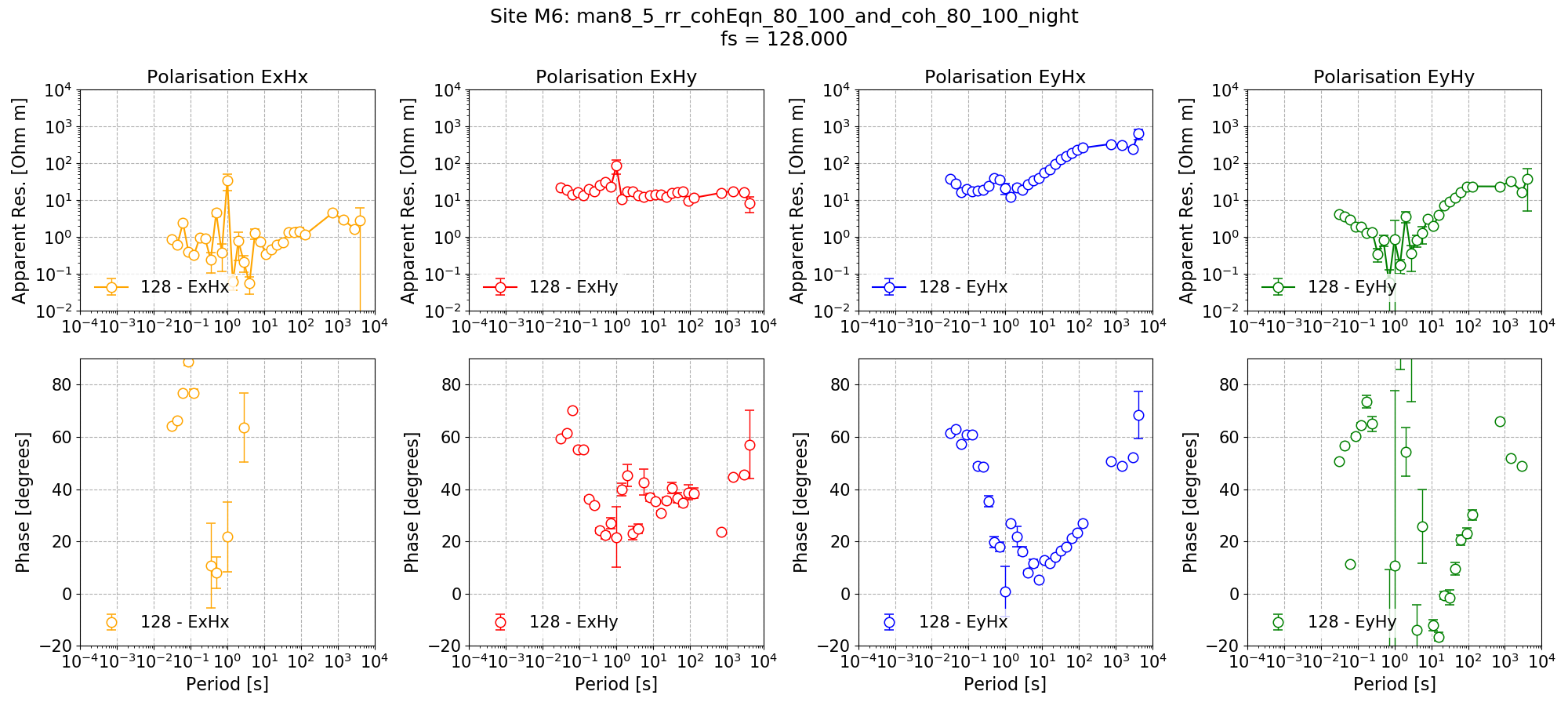
Remote reference impedance tensor estimates for Site M6 at 128 Hz using 8 decimation levels and 5 evaluation frequencies per level with a custom window size per decimation level. Masks and time constraints are applied. An additional mask is applied for Remote excluding Remote windows with coherence Ex-Hy or Ey-Hx below 0.8.
The result here is not so good, but it has reduced the biasing in the dead band where previously phases were reaching 0. With extra work and configuration testing, this may be promising.
For a last try, variable single site coherence thresholds could be used to limit the Remote data using the addConstraintLevel() method of MaskData. An example and the result are provided below.
125 126 127 128 129 130 131 132 133 134 135 136 137 138 139 140 141 142 143 144 145 146 147 148 149 150 151 152 153 154 155 156 157 158 159 | # try one more where the Remote coherence mask is variable to avoid losing two many windows and long periods
maskData = newMaskData(proj, 128)
maskData.setStats(["coherence"])
maskData.addConstraintLevel("coherence", {"cohExHy": [0.9, 1.0], "cohEyHx": [0.9, 1.0]}, 0)
maskData.addConstraintLevel("coherence", {"cohExHy": [0.8, 1.0], "cohEyHx": [0.8, 1.0]}, 1)
maskData.addConstraintLevel("coherence", {"cohExHy": [0.5, 1.0], "cohEyHx": [0.5, 1.0]}, 2)
maskData.addConstraintLevel("coherence", {"cohExHy": [0.3, 1.0], "cohEyHx": [0.3, 1.0]}, 3)
maskData.addConstraintLevel("coherence", {"cohExHy": [0.2, 1.0], "cohEyHx": [0.2, 1.0]}, 4)
# finally, lets give maskData a name, which will relate to the output file
maskData.maskName = "coh_variable"
calculateMask(proj, maskData, sites=["M6", "Remote"])
maskData.printInfo()
processProject(
proj,
sites=["M6"],
sampleFreqs=[128],
remotesite="Remote",
masks={"M6": ["rr_cohEqn_80_100"], "Remote": "coh_variable"},
datetimes=[
{"type": "time", "start": "20:00:00", "stop": "07:00:00", "levels": [0, 1]}
],
postpend="rr_cohEqn_80_100_and_coh_variable_night",
)
figs = viewImpedance(
proj,
sites=["M6"],
sampleFreqs=[128],
postpend="rr_cohEqn_80_100_and_coh_variable_night",
oneplot=False,
plotoptions=plotOptions,
save=False,
show=False,
)
figs[0].savefig(remoteImages / "remoteReferenceM6_128_RR_man8_5_cohvar_datetime_01.png")
|
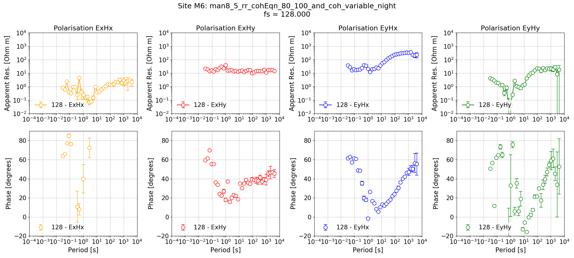
Remote reference impedance tensor estimates for Site M6 at 128 Hz using 8 decimation levels and 5 evaluation frequencies per level with a custom window size per decimation level. Masks and time constraints are applied. An additional mask is applied for Remote excluding Remote windows with coherence Ex-Hy or Ey-Hx below thresholds which are specified individually for each decimation level.
Note
The data for this example has come from a field survey of northern Switzerland in 2016. This data is explored in more detail in a case study.
Complete example scripts
For the purposes of clarity, the complete example scripts are provided below.
Configuration dec8_5:
1 2 3 4 5 6 7 8 9 10 11 12 13 14 15 16 17 18 19 20 21 22 23 24 25 26 27 28 29 30 31 32 33 34 35 36 37 38 39 40 41 42 43 44 45 46 47 48 49 50 51 52 53 54 55 56 57 58 59 60 61 62 63 64 65 66 67 | from datapaths import remotePath, remoteImages
from resistics.project.io import loadProject
from resistics.project.spectra import calculateSpectra
from resistics.project.transfunc import processProject, viewImpedance
from resistics.project.statistics import calculateRemoteStatistics, viewStatistic
from resistics.project.mask import newMaskData, calculateMask
from resistics.common.plot import plotOptionsTransferFunction, getPaperFonts
plotOptions = plotOptionsTransferFunction(plotfonts=getPaperFonts())
proj = loadProject(remotePath, "remoteConfig.ini")
calculateSpectra(proj, sites=["M6", "Remote"])
proj.refresh()
# single site processing
processProject(proj, sites=["M6", "Remote"])
figs = viewImpedance(
proj,
sites=["M6", "Remote"],
sampleFreqs=[128],
oneplot=False,
plotoptions=plotOptions,
save=False,
show=False,
)
figs[0].savefig(remoteImages / "singleSiteM6_128_dec8_5.png")
figs[1].savefig(remoteImages / "singleSiteRemote_128_dec8_5.png")
# calculate the statistic we are interested in
calculateRemoteStatistics(proj, "Remote", sites=["M6"], sampleFreqs=[128])
# generate mask
maskData = newMaskData(proj, 128)
maskData.setStats(["RR_coherenceEqn"])
maskData.addConstraint(
"RR_coherenceEqn", {"ExHyR-HyHyR": [0.8, 1.0], "EyHxR-HxHxR": [0.8, 1.0]}
)
# finally, lets give maskData a name, which will relate to the output file
maskData.maskName = "rr_cohEqn_80_100"
calculateMask(proj, maskData, sites=["M6"])
maskData.printInfo()
# process with masks
processProject(
proj,
sites=["M6"],
sampleFreqs=[128],
remotesite="Remote",
masks={"M6": "rr_cohEqn_80_100"},
datetimes=[
{"type": "time", "start": "20:00:00", "stop": "07:00:00", "levels": [0, 1]}
],
postpend="rr_cohEqn_80_100_night",
)
figs = viewImpedance(
proj,
sites=["M6"],
sampleFreqs=[128],
postpend="rr_cohEqn_80_100_night",
oneplot=False,
plotoptions=plotOptions,
save=False,
show=False,
)
figs[0].savefig(remoteImages / "remoteReferenceM6_128_RR_dec8_5_coh_datetime_01.png")
|
Configuration man8_5:
1 2 3 4 5 6 7 8 9 10 11 12 13 14 15 16 17 18 19 20 21 22 23 24 25 26 27 28 29 30 31 32 33 34 35 36 37 38 39 40 41 42 43 44 45 46 47 48 49 50 51 52 53 54 55 56 57 58 59 60 61 62 63 64 65 66 67 68 69 70 71 72 73 74 75 76 77 78 79 80 81 82 83 84 85 86 87 88 89 90 91 92 93 94 95 96 97 98 99 100 101 102 103 104 105 106 107 108 109 110 111 112 113 114 115 116 117 118 119 120 121 122 123 124 125 126 127 128 129 130 131 132 133 134 135 136 137 138 139 140 141 142 143 144 145 146 147 148 149 150 151 152 153 154 155 156 157 158 159 | from datapaths import remotePath, remoteImages
from resistics.project.io import loadProject
from resistics.project.spectra import calculateSpectra
from resistics.project.transfunc import processProject, viewImpedance
from resistics.project.statistics import (
calculateStatistics,
calculateRemoteStatistics,
viewStatistic,
)
from resistics.project.mask import newMaskData, calculateMask
from resistics.common.plot import plotOptionsTransferFunction, getPaperFonts
plotOptions = plotOptionsTransferFunction(plotfonts=getPaperFonts())
proj = loadProject(remotePath, "manualWindowsConfig.ini")
# calculate spectra
calculateSpectra(proj, sites=["M6", "Remote"])
proj.refresh()
processProject(proj, sites=["M6", "Remote"])
figs = viewImpedance(
proj,
sites=["M6", "Remote"],
sampleFreqs=[128],
oneplot=False,
plotoptions=plotOptions,
save=False,
show=False,
)
figs[0].savefig(remoteImages / "singleSiteM6_128_man8_5.png")
figs[1].savefig(remoteImages / "singleSiteRemote_128_man8_5.png")
# calculate the statistic we are interested in
calculateStatistics(proj, sites=["M6", "Remote"], sampleFreqs=[128])
calculateRemoteStatistics(proj, "Remote", sites=["M6"], sampleFreqs=[128])
# generate single site masks
maskData = newMaskData(proj, 128)
maskData.setStats(["coherence"])
maskData.addConstraint("coherence", {"cohExHy": [0.8, 1.0], "cohEyHx": [0.8, 1.0]})
# finally, lets give maskData a name, which will relate to the output file
maskData.maskName = "coh_80_100"
calculateMask(proj, maskData, sites=["M6", "Remote"])
maskData.printInfo()
# process remote on its own to compare to the first processing we did
processProject(
proj,
sites=["Remote"],
sampleFreqs=[128],
masks={"Remote": "coh_80_100"},
postpend="coh_80_100",
)
figs = viewImpedance(
proj,
sites=["Remote"],
sampleFreqs=[128],
postpend="coh_80_100",
oneplot=False,
plotoptions=plotOptions,
save=False,
show=False,
)
figs[0].savefig(remoteImages / "singleSiteRemote_128_man8_5_coh80.png")
# generate mask
maskData = newMaskData(proj, 128)
maskData.setStats(["RR_coherenceEqn"])
maskData.addConstraint(
    "RR_coherenceEqn", {"ExHyR-HyHyR": [0.8, 1.0], "EyHxR-HxHxR": [0.8, 1.0]}
)
# finally, lets give maskData a name, which will relate to the output file
maskData.maskName = "rr_cohEqn_80_100"
calculateMask(proj, maskData, sites=["M6"])
maskData.printInfo()

# process with masks
processProject(
    proj,
    sites=["M6"],
    sampleFreqs=[128],
    remotesite="Remote",
    masks={"M6": "rr_cohEqn_80_100"},
    datetimes=[
        {"type": "time", "start": "20:00:00", "stop": "07:00:00", "levels": [0, 1]}
    ],
    postpend="rr_cohEqn_80_100_night",
)
figs = viewImpedance(
    proj,
    sites=["M6"],
    sampleFreqs=[128],
    postpend="rr_cohEqn_80_100_night",
    oneplot=False,
    plotoptions=plotOptions,
    save=False,
    show=False,
)
figs[0].savefig(remoteImages / "remoteReferenceM6_128_RR_man8_5_coh_datetime_01.png")
# one more example with multiple masks
# let's use standard coherence as well for Remote only
processProject(
    proj,
    sites=["M6"],
    sampleFreqs=[128],
    remotesite="Remote",
    masks={"M6": ["rr_cohEqn_80_100"], "Remote": "coh_80_100"},
    datetimes=[
        {"type": "time", "start": "20:00:00", "stop": "07:00:00", "levels": [0, 1]}
    ],
    postpend="rr_cohEqn_80_100_and_coh_80_100_night",
)
figs = viewImpedance(
    proj,
    sites=["M6"],
    sampleFreqs=[128],
    postpend="rr_cohEqn_80_100_and_coh_80_100_night",
    oneplot=False,
    plotoptions=plotOptions,
    save=False,
    show=False,
)
figs[0].savefig(remoteImages / "remoteReferenceM6_128_RR_man8_5_2coh_datetime_01.png")
# try one more where the Remote coherence mask is variable to avoid losing two many windows and long periods
maskData = newMaskData(proj, 128)
maskData.setStats(["coherence"])
maskData.addConstraintLevel("coherence", {"cohExHy": [0.9, 1.0], "cohEyHx": [0.9, 1.0]}, 0)
maskData.addConstraintLevel("coherence", {"cohExHy": [0.8, 1.0], "cohEyHx": [0.8, 1.0]}, 1)
maskData.addConstraintLevel("coherence", {"cohExHy": [0.5, 1.0], "cohEyHx": [0.5, 1.0]}, 2)
maskData.addConstraintLevel("coherence", {"cohExHy": [0.3, 1.0], "cohEyHx": [0.3, 1.0]}, 3)
maskData.addConstraintLevel("coherence", {"cohExHy": [0.2, 1.0], "cohEyHx": [0.2, 1.0]}, 4)
# finally, lets give maskData a name, which will relate to the output file
maskData.maskName = "coh_variable"
calculateMask(proj, maskData, sites=["M6", "Remote"])
maskData.printInfo()

processProject(
    proj,
    sites=["M6"],
    sampleFreqs=[128],
    remotesite="Remote",
    masks={"M6": ["rr_cohEqn_80_100"], "Remote": "coh_variable"},
    datetimes=[
        {"type": "time", "start": "20:00:00", "stop": "07:00:00", "levels": [0, 1]}
    ],
    postpend="rr_cohEqn_80_100_and_coh_variable_night",
)
figs = viewImpedance(
    proj,
    sites=["M6"],
    sampleFreqs=[128],
    postpend="rr_cohEqn_80_100_and_coh_variable_night",
    oneplot=False,
    plotoptions=plotOptions,
    save=False,
    show=False,
)
figs[0].savefig(remoteImages / "remoteReferenceM6_128_RR_man8_5_cohvar_datetime_01.png")
|