Pre-processing timeseries data
There are scenarios in which time series data must be pre-processed and saved before transfer function calculation. Pre-processing is predominantly performed in the project environment using the preProcess() method. There are several pre-processing options available in preProcess() method, including:
Another preprocessing method of use, but not available within the preProcess() method is gap filling. This can help increase the number of windows at long periods.
In addition, there are lower levels APIs for performing these actions for advanced users. Please see the API doc for more information or check the Cookbook.
The preprocessing options are explained in more detail below. The data is the same 4096 Hz data from the tutorial and is saved in “site1”. A project has already been setup following the instructions in Project environment. In all the following, the project has already been loaded as shown below.
1 2 3 4 5 | from datapaths import preprocessPath, preprocessImages
from resistics.project.io import loadProject
proj = loadProject(preprocessPath)
proj.printInfo()
|
For plotting the time data, different plot options are used to give larger fonts. Plot fonts have been defined as follows:
7 8 | from resistics.common.plot import plotOptionsTime, getPresentationFonts
plotOptions = plotOptionsTime(plotfonts=getPresentationFonts())
|
Data resampling
Resampling time series data might be required to ensure matching sampling rates between different datasets, for example a local site and a reference site. This can be achieved through the resampling option in preProcess() method which can save the data either to the same site or to a new site altogether.
Below is an exampling of downsampling a 4096 Hz dataset to 1024 Hz. The output will be saved to a new site named “site1_resample”. If the site does not already exist, it will be created. The name of the measurement in the new site will be:
Note
prepend + meas_[start_time] + postpend give an example
As the measurement is being written out to a new site, prepend is being set “” (an empty string). By default, postpend is an empty string.
10 11 12 13 14 15 16 17 18 19 20 21 22 23 24 25 26 27 28 29 30 31 | # resample to 1024 Hz and save in new site
from resistics.project.time import preProcess
preProcess(
proj, sites="site1", resamp={4096: 1024}, outputsite="site1_resample", prepend=""
)
proj.refresh()
proj.printInfo()
# let's view the time series
from resistics.project.time import viewTime
fig = viewTime(
proj,
"2012-02-10 11:05:00",
"2012-02-10 11:05:03",
sites=["site1", "site1_resample"],
chans=["Hx", "Hy", "Hz"],
show=False,
plotoptions=plotOptions,
)
fig.savefig(preprocessImages / "viewTimeResample.png")
|
These produce the following plots:
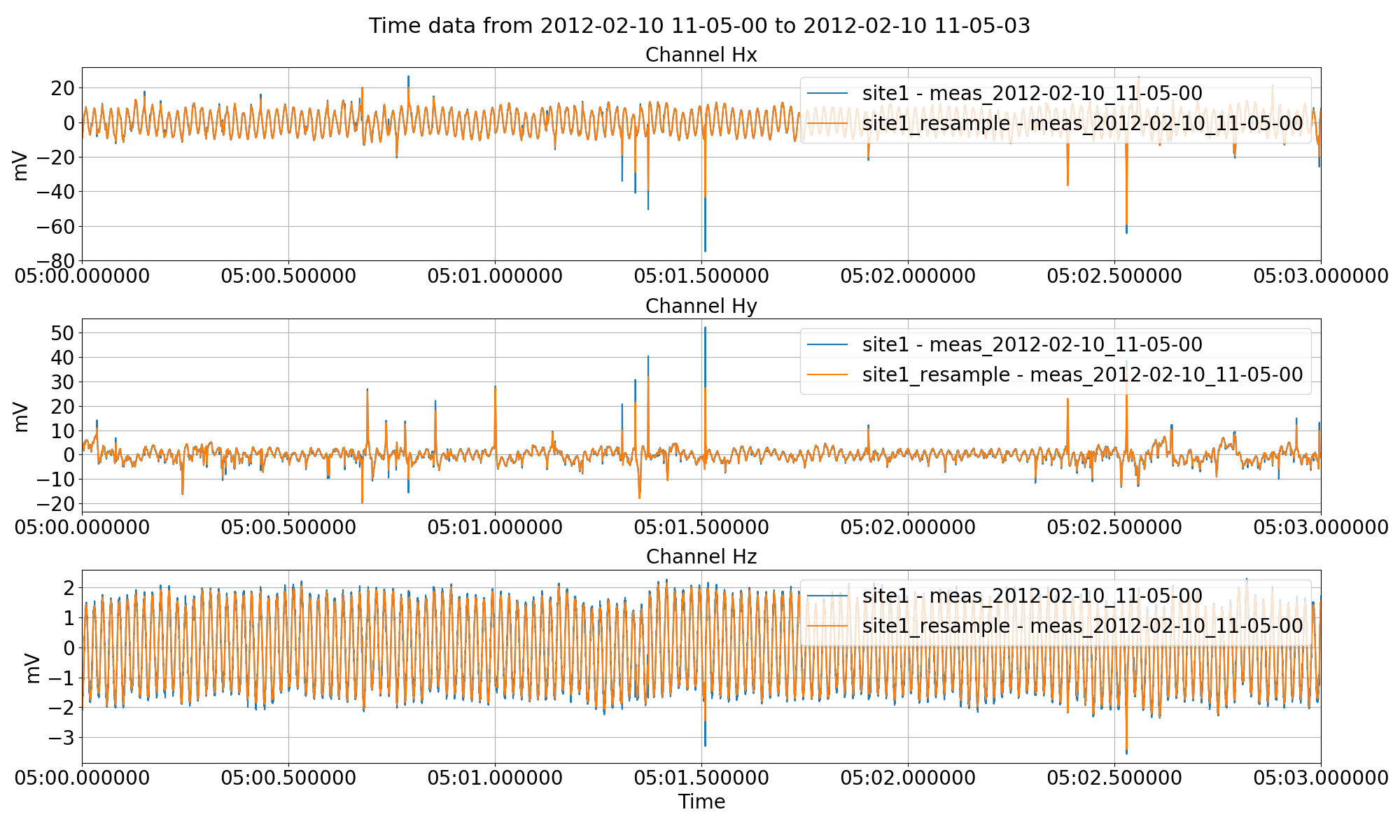
Resampling data from 4096 Hz to 1024 Hz example using the preProcess() method.
Polarity reversal
This simply multiples the requested channels by -1. This is particularly useful when electric channels have been connected in the opposite way. An example is shown below of the polarity reversal of an electric channel.
10 11 12 13 14 15 16 17 18 19 20 21 22 23 24 25 26 27 28 29 30 31 32 | # polarity reverse the Ey channel
from resistics.project.time import preProcess, viewTime
preProcess(
proj,
sites="site1",
polreverse={"Ey": True},
outputsite="site1_polreverse",
prepend="",
)
proj.refresh()
proj.printInfo()
fig = viewTime(
proj,
"2012-02-10 11:05:00",
"2012-02-10 11:05:01",
sites=["site1", "site1_polreverse"],
chans=["Ex", "Ey"],
show=False,
plotoptions=plotOptions,
)
fig.savefig(preprocessImages / "viewTimePolarityReversal.png")
|
The results of this can be seen in the following figure.
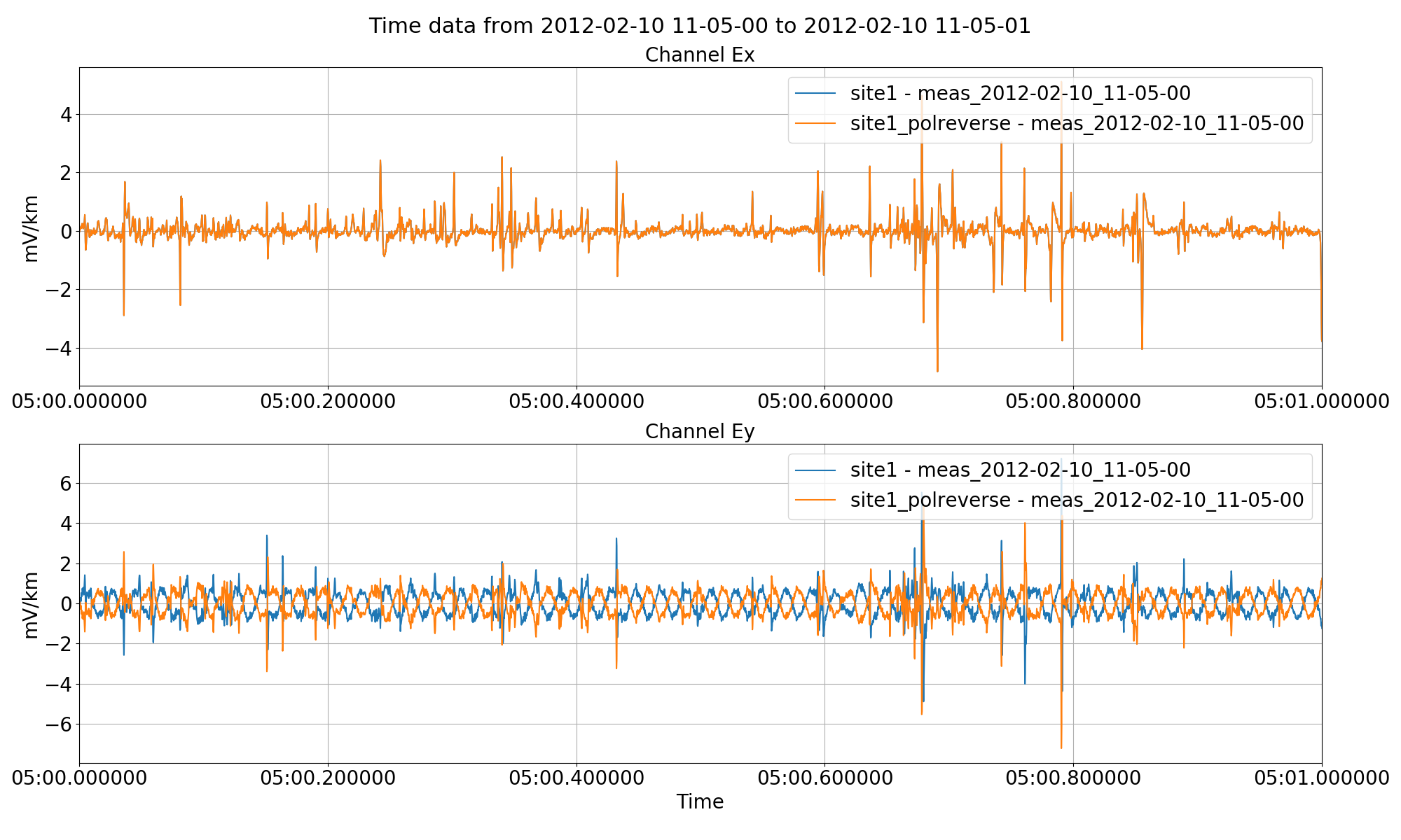
Polarity reversal for channel Ey using the preProcess() method.
Scaling
If more arbitrary scaling control is required than simply multiplying by -1, the scale option of preProcess() can be used.
34 35 36 37 38 39 40 41 42 43 44 45 46 47 48 49 50 51 52 53 | preProcess(
proj,
sites="site1",
scale={"Ex": -2, "Ey": 0.5},
outputsite="site1_scale",
prepend="",
)
proj.refresh()
proj.printInfo()
fig = viewTime(
proj,
"2012-02-10 11:05:00",
"2012-02-10 11:05:01",
sites=["site1", "site1_scale"],
chans=["Ex", "Ey"],
show=False,
plotoptions=plotOptions,
)
fig.savefig(preprocessImages / "viewTimeScale.png")
|
This will scale the Ex channel by -2 and the Ey channel by 0.5.
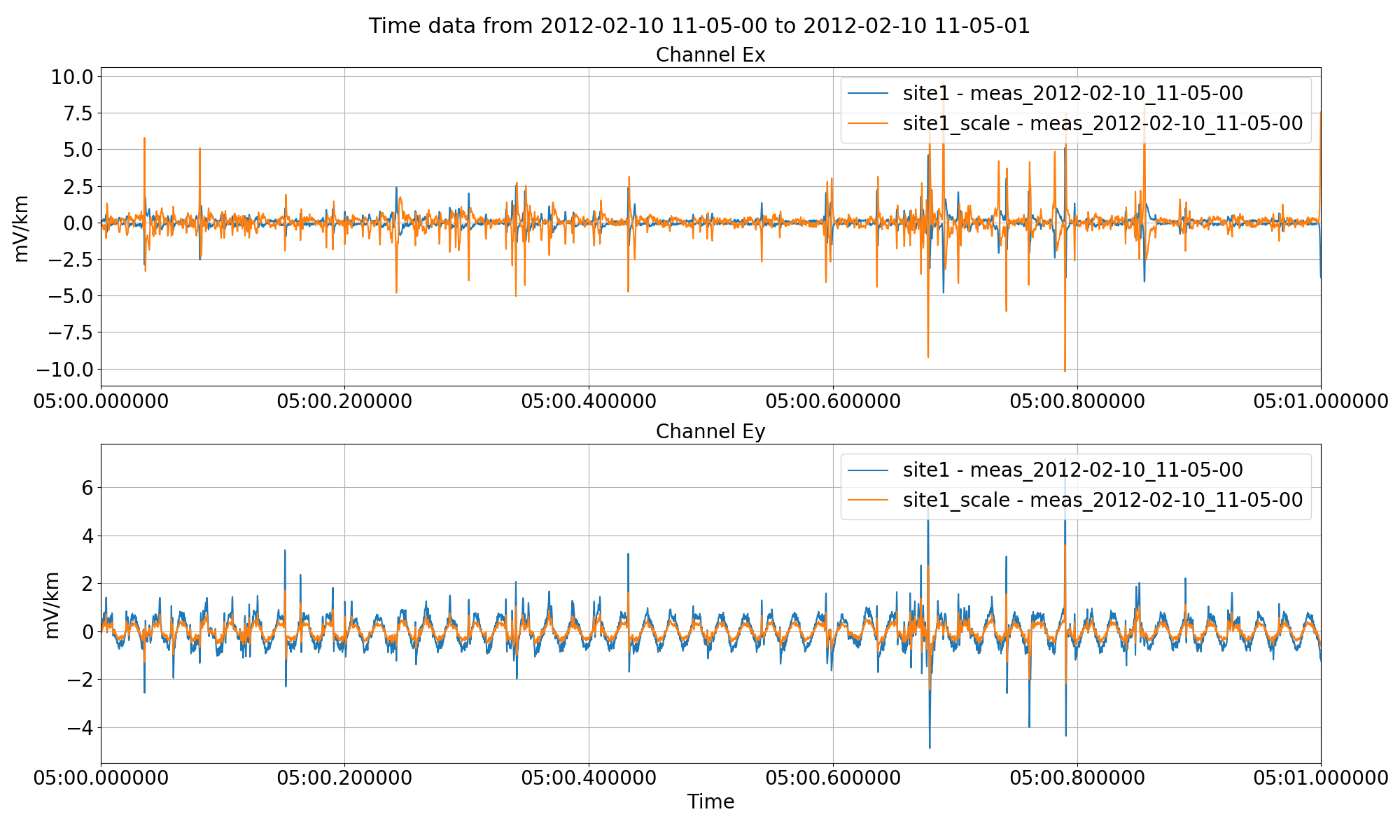
Scaling channel Ex by -2 and Ey by 0.5 using the scale option of the preProcess() method.
Calibration
The data can be pre-calibrated in a situation where calibrated time series data is required for viewing, exporting or other purposes. For example, data can be calibrated in resistics and then further processing can be done using other tools as required. To perform calibration, the calibration files need to be present in the calData folder of the project. For more information on calibration files, please see the Calibration information in the Data formats section.
Below is an example of calibrating time series:
83 84 85 86 87 88 89 90 91 92 93 94 95 96 97 98 | preProcess(
proj, sites="site1", calibrate=True, outputsite="site1_calibrate", prepend=""
)
proj.refresh()
proj.printInfo()
fig = viewTime(
proj,
"2012-02-10 11:05:00",
"2012-02-10 11:05:03",
sites=["site1", "site1_calibrate"],
chans=["Ex", "Hx"],
show=False,
plotoptions=plotOptions,
)
fig.savefig(preprocessImages / "viewTimeCalibrate.png")
|
This will calibrate the magnetic channels in the data, converting them from mV to nT.
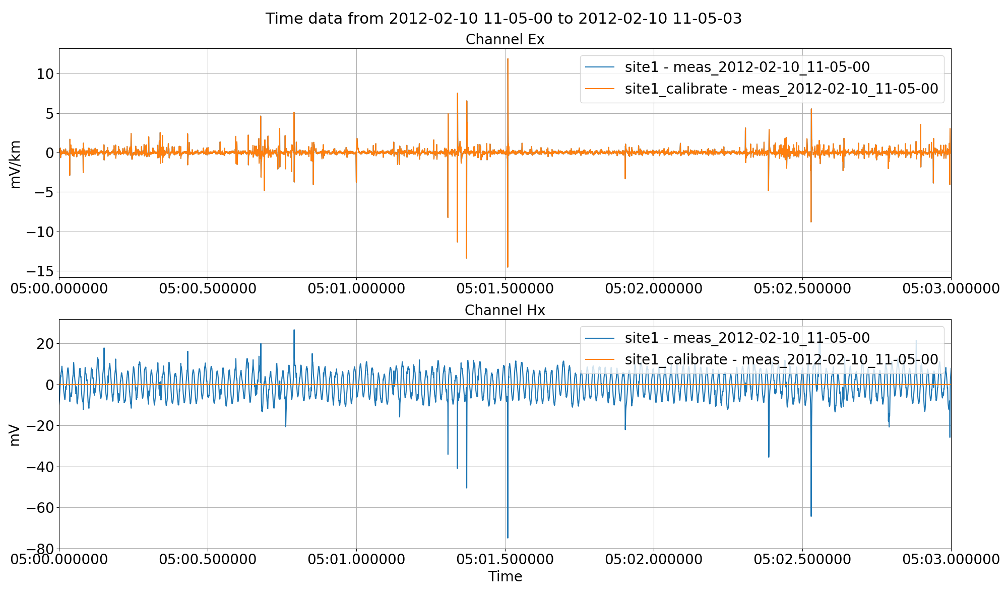
Calibrating the magnetic channels of the data using the calibration option of the preProcess() method.
Low, band and high pass filtering
Time series data can be low, band and high pass filtered as required. This normally useful for viewing but can be useful for exporting or other purposes. Filter options can be specified in Hz using the filter keyword to the preProcess() method. The keyword expects a dictionary with various filter options such as:
lpfilt : low pass filtering
hpfilt : high pass filtering
bpfilt : band pass filtering
Examples of each are provided below.
Low pass filtering using the lpfilt option to filter 4096 Hz to 32 Hz (without impacting the sampling rate).
10 11 12 13 14 15 16 17 18 19 20 21 22 23 24 25 26 27 28 | # resample to 1024 Hz and save in new site
from resistics.project.time import preProcess, viewTime
preProcess(
proj, sites="site1", filter={"lpfilt": 32}, outputsite="site1_lowpass", prepend=""
)
proj.refresh()
proj.printInfo()
fig = viewTime(
proj,
"2012-02-10 11:05:00",
"2012-02-10 11:05:03",
sites=["site1", "site1_lowpass"],
chans=["Hx", "Hy", "Hz"],
show=False,
plotoptions=plotOptions,
)
fig.savefig(preprocessImages / "viewTimeLowpass.png")
|
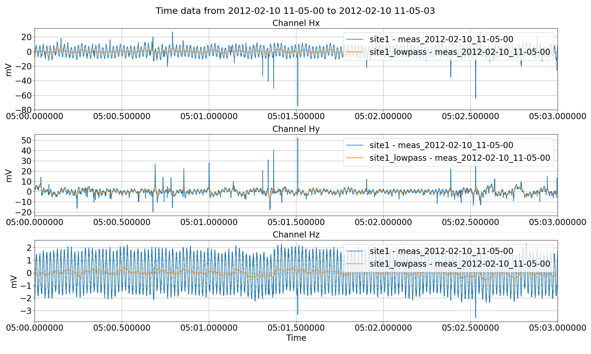
Low pass filtering the time series data and saving it out to another site using the filter keyword to the preProcess() method.
Highpass filtering can be specified in a similar way.
30 31 32 33 34 35 36 37 38 39 40 41 42 43 44 45 | preProcess(
proj, sites="site1", filter={"hpfilt": 512}, outputsite="site1_highpass", prepend=""
)
proj.refresh()
proj.printInfo()
fig = viewTime(
proj,
"2012-02-10 11:05:00",
"2012-02-10 11:05:03",
sites=["site1", "site1_highpass"],
chans=["Hx", "Hy", "Hz"],
show=False,
plotoptions=plotOptions,
)
fig.savefig(preprocessImages / "viewTimeHighpass.png")
|
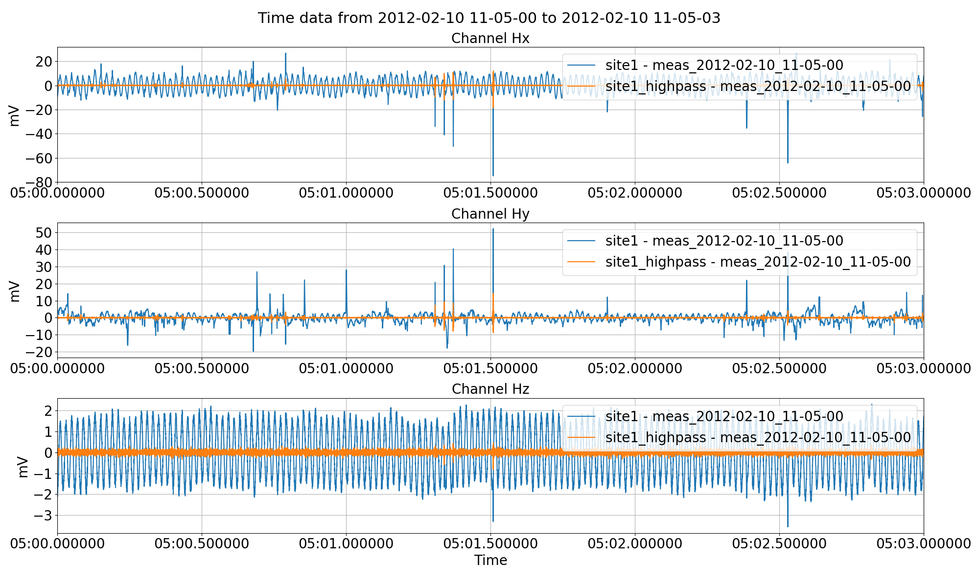
High pass filtering the time series data and saving it out to another site using the filter keyword to the preProcess() method.
Band pass filtering can performed as follows:
47 48 49 50 51 52 53 54 55 56 57 58 59 60 61 62 63 64 65 66 | preProcess(
proj,
sites="site1",
filter={"bpfilt": [100, 2000]},
outputsite="site1_bandpass",
prepend="",
)
proj.refresh()
proj.printInfo()
fig = viewTime(
proj,
"2012-02-10 11:05:00",
"2012-02-10 11:05:03",
sites=["site1", "site1_bandpass"],
chans=["Hx", "Hy", "Hz"],
show=False,
plotoptions=plotOptions,
)
fig.savefig(preprocessImages / "viewTimeBandpass.png")
|
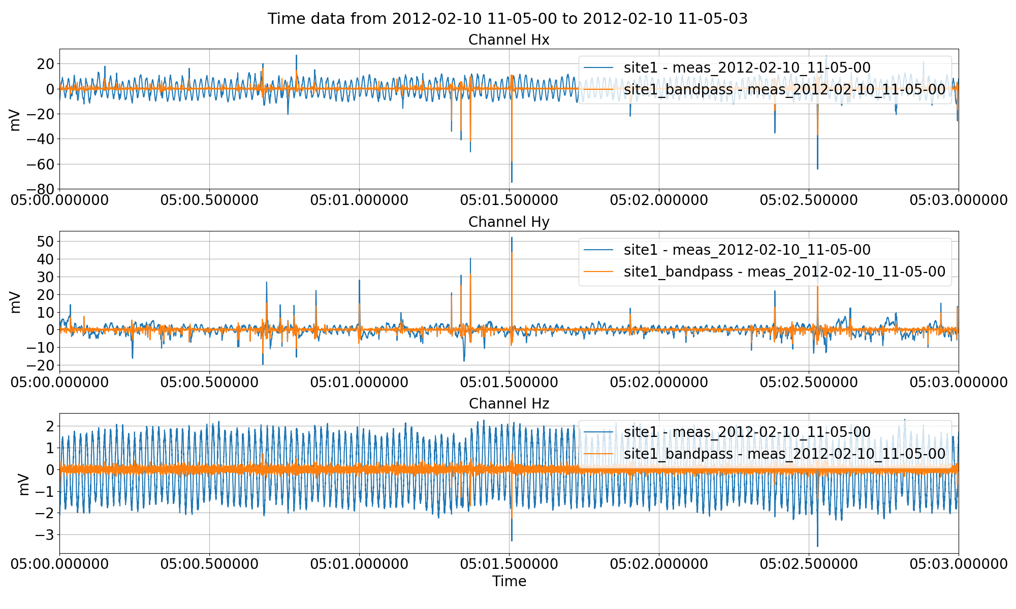
Band pass filtering the time series data and saving it out to another site using the filter keyword to the preProcess() method. Unlike high pass or low pass filtering, two frequencies need to provided, one defining the low cut and the other, the high cut.
Notch filter
Notch filters are useful ways to remove unwanted signal in data. The most common frequency domain noise spikes which may need filtering are powerline noise or railway noise at 50 Hz and 16.6 Hz respectively. Notching frequencies are specified in Hz using the notch keyword to the preProcess() method. This is expected to be a list of frequencies to notch in Hz.
An example is given below of removing 50 Hz from time series data.
68 69 70 71 72 73 74 75 76 77 78 79 80 81 | preProcess(proj, sites="site1", notch=[50], outputsite="site1_notch", prepend="")
proj.refresh()
proj.printInfo()
fig = viewTime(
proj,
"2012-02-10 11:05:00",
"2012-02-10 11:05:03",
sites=["site1", "site1_notch"],
chans=["Hx", "Hy", "Hz"],
show=False,
plotoptions=plotOptions,
)
fig.savefig(preprocessImages / "viewTimeNotch.png")
|
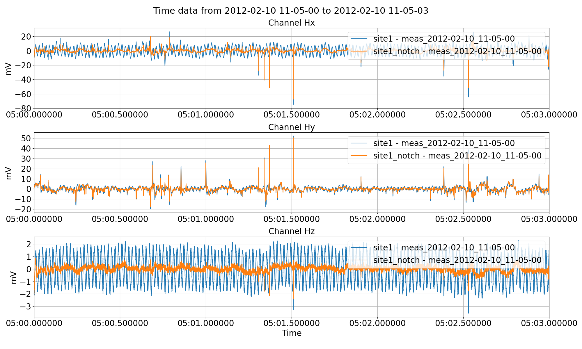
Notch filtering the time series data and saving it out to another site using the notch keyword to the preProcess() method.
Data normalisation
Data normalisation normalises the data by diving by the norm of the data as calculated by numpy norm. There are few practical uses for this, though it may be of interest for other analytics based on the time series data.
55 56 57 58 59 60 61 62 63 64 65 66 67 68 69 70 71 72 73 74 75 | # normalisation
preProcess(
proj,
sites="site1",
normalise=True,
outputsite="site1_norm",
prepend="",
)
proj.refresh()
proj.printInfo()
fig = viewTime(
proj,
"2012-02-10 11:05:00",
"2012-02-10 11:05:01",
sites=["site1", "site1_norm"],
chans=["Ex", "Ey"],
show=False,
plotoptions=plotOptions,
)
fig.savefig(preprocessImages / "viewTimeNorm.png")
|
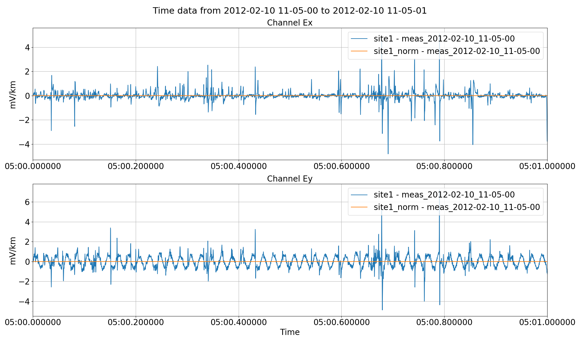
Normalising the time series data and saving it out to another site using the normalise keyword to the preProcess() method.
Interpolation to second
Resistics assumes that data is sampled on the second. For more information on this, please see time series formats and interpolation to second.
Gap filling
In some situations, it is beneficial to stitch together two separate time series to increase the number of windows at long periods. This can be done through gap filling. However, resistics gap filling is external to the preProcess() method and has to be specified using other APIs.
To see an example, begin by saving smaller pieces of data from site1. Here, two smaller subsets are being saved to the same site, “site1_gaps”. To understand more about data readers in resistics, please see time series formats.
12 13 14 15 16 17 18 19 20 21 22 23 24 25 26 27 28 29 30 31 32 33 34 35 36 37 38 39 40 41 42 43 44 45 46 47 48 49 50 51 52 53 54 55 | from resistics.time.reader_ats import TimeReaderATS
site1 = proj.getSiteData("site1")
readerATS = TimeReaderATS(site1.getMeasurementTimePath("meas_2012-02-10_11-05-00"))
# headers of recording
headers = readerATS.getHeaders()
chanHeaders, chanMap = readerATS.getChanHeaders()
# separate out two datasets
timeOriginal1 = readerATS.getPhysicalData(
"2012-02-10 11:05:00", "2012-02-10 11:09:00", remaverage=False
)
timeOriginal2 = readerATS.getPhysicalData(
"2012-02-10 11:10:00", "2012-02-10 11:14:00", remaverage=False
)
from resistics.time.writer_internal import TimeWriterInternal
# create a new site
proj.createSite("site1_gaps")
proj.refresh()
writer = TimeWriterInternal()
writer.setOutPath(
Path(proj.timePath, "site1_gaps", "meas_2012-02-10_11-05-00_section1")
)
writer.writeData(headers, chanHeaders, timeOriginal1, physical=True)
writer.setOutPath(
Path(proj.timePath, "site1_gaps", "meas_2012-02-10_11-05-00_section2")
)
writer.writeData(headers, chanHeaders, timeOriginal2, physical=True)
from resistics.project.time import viewTime
# now view time
fig = viewTime(
proj,
"2012-02-10 11:05:00",
"2012-02-10 11:14:00",
sites=["site1", "site1_gaps"],
filter={"lpfilt": 16},
chans=["Ex", "Hy"],
show=False,
plotoptions=plotOptions,
)
fig.savefig(preprocessImages / "viewTimeGaps.png")
|
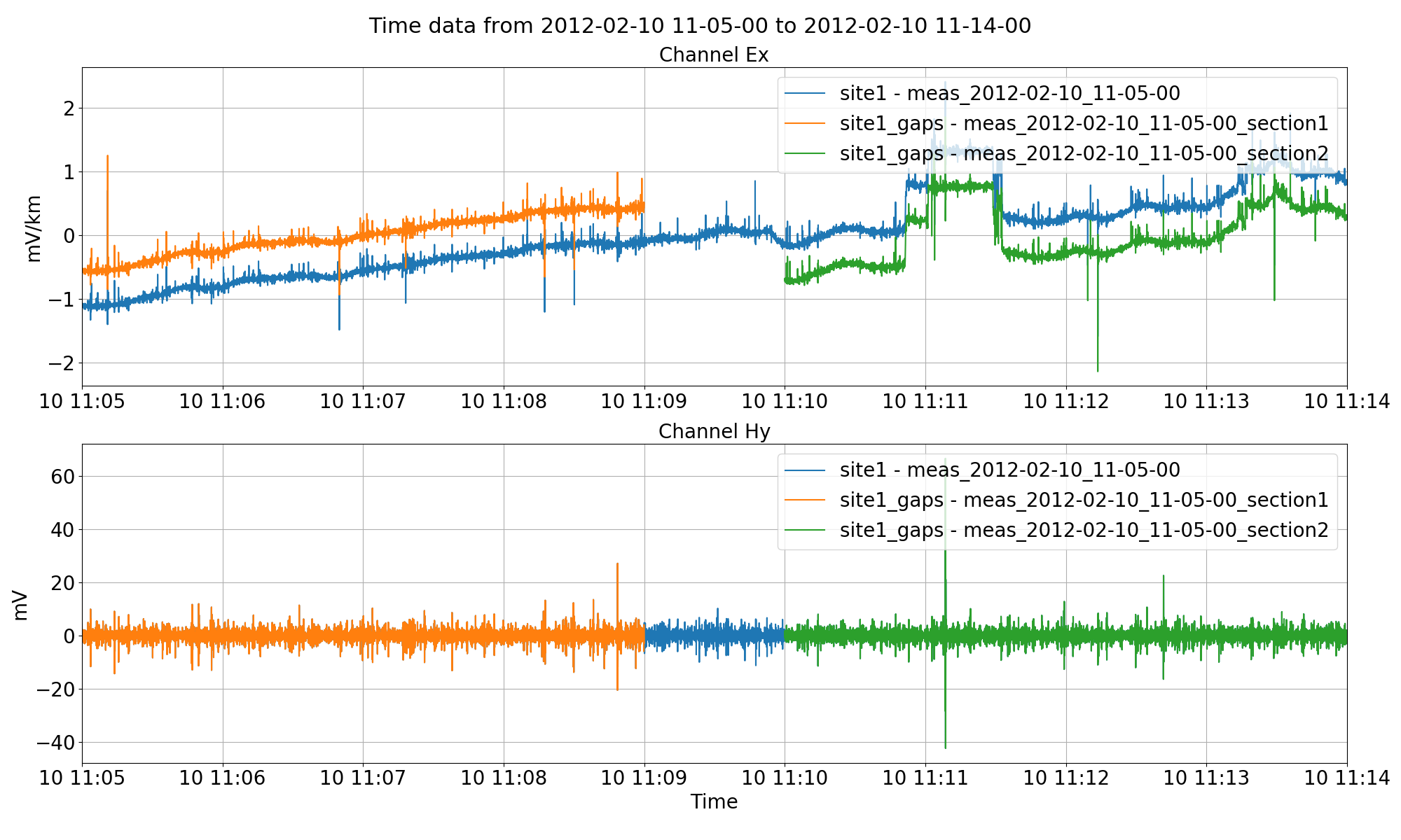
Splitting up site1 data into two smaller measurements in a new site named “site1_gaps”. Note, for the electric channel, the data does not sit on top of each other because the mean is being removed from all the measurements independently for visualisation.
It is important at this stage not to remove the mean when getting the time data. Removing the mean will remove separate means for the independent sub time series as can be seen in the above figure. Mean is removed automatically for visualisation when using the viewTime() method. However, by specifying when getting the time data that remaverage=False, the underlying data will still have the original average when written out.
The next stage is to read the separate data in as TimeData objects by using the TimeReaderInternal class.
57 58 59 60 61 62 63 64 65 66 67 68 69 70 | from resistics.time.reader_internal import TimeReaderInternal
siteGaps = proj.getSiteData("site1_gaps")
readerSection1 = TimeReaderInternal(
siteGaps.getMeasurementTimePath("meas_2012-02-10_11-05-00_section1")
)
timeData1 = readerSection1.getPhysicalSamples(remaverage=False)
timeData1.printInfo()
readerSection2 = TimeReaderInternal(
siteGaps.getMeasurementTimePath("meas_2012-02-10_11-05-00_section2")
)
timeData2 = readerSection2.getPhysicalSamples(remaverage=False)
timeData2.printInfo()
|
The two separate datasets can be stitched together using the fillGap() method of module interp.
68 69 70 71 72 73 74 | from resistics.time.interp import fillGap
timeDataFilled = fillGap(timeData1, timeData2)
timeDataFilled.printInfo()
samplesToView = 14 * 60 * 4096
fig = timeDataFilled.view(sampleStop=samplesToView, chans=["Ex", "Hy"])
fig.savefig(preprocessImages / "timeDataFilled.png")
|
The filled time data can be viewed using the view() method of the TimeData class.
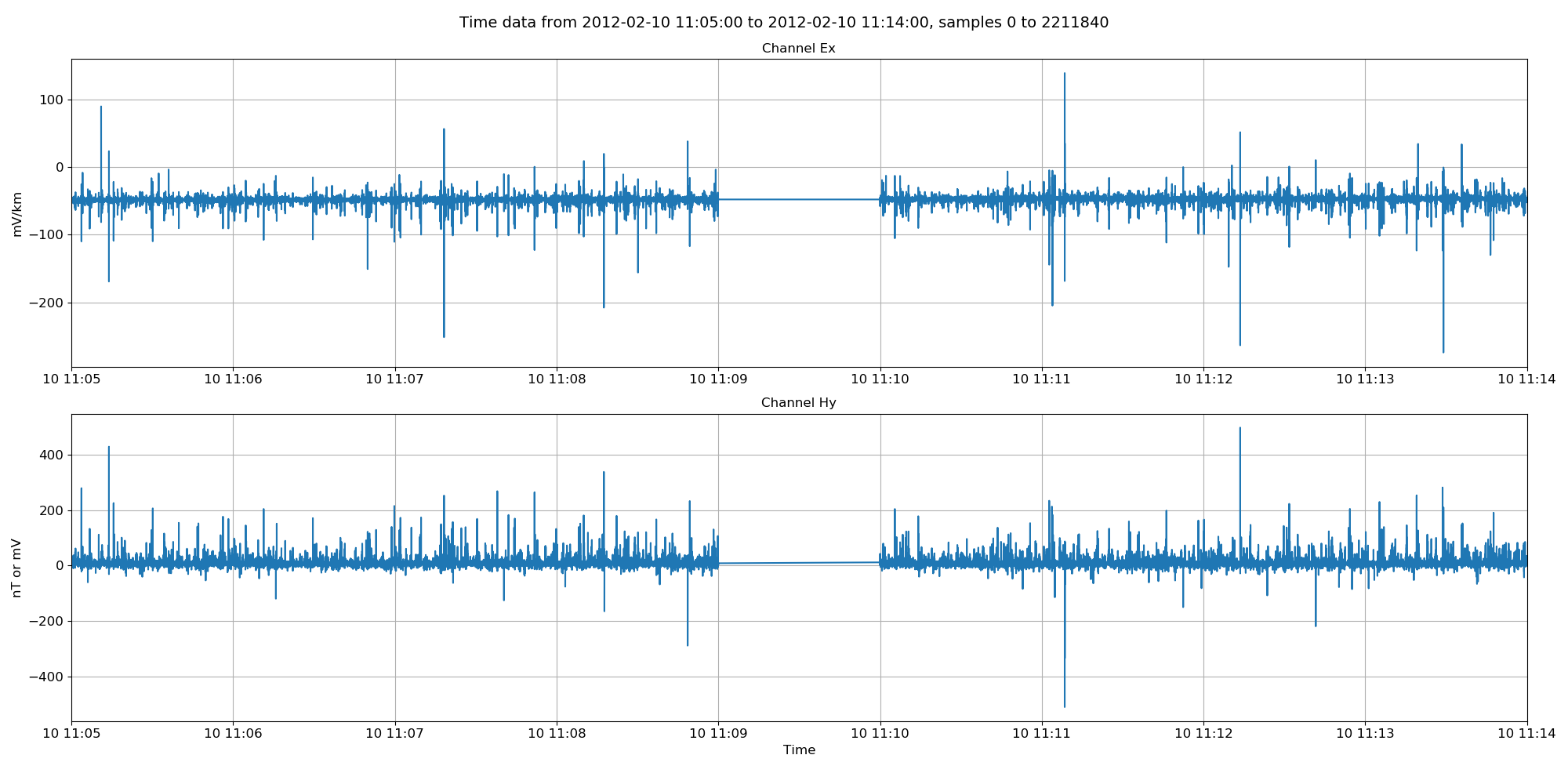
The filled time data. The missing points have now been filled in linearly between the two datasets. Note, this data is not low pass filtered like in the previous plot.
Now the data can be written out using the TimeWriterInternal class.
80 81 82 83 84 85 86 87 88 89 90 91 | # create a new site to write out to
proj.createSite("site1_filled")
proj.refresh()
# use channel headers from one of the datasets, stop date will be automatically amended
writer = TimeWriterInternal()
writer.setOutPath(
Path(proj.timePath, "site1_filled", "meas_2012-02-10_11-05-00_filled")
)
headers = readerSection1.getHeaders()
chanHeaders, chanMap = readerSection1.getChanHeaders()
writer.writeData(headers, chanHeaders, timeDataFilled, physical=True)
proj.refresh()
|
Finally, view the new site with filled time data compared to the original.
93 94 95 96 97 98 99 100 101 102 103 104 | # now view time
fig = viewTime(
proj,
"2012-02-10 11:05:00",
"2012-02-10 11:14:00",
sites=["site1", "site1_filled"],
filter={"lpfilt": 16},
chans=["Ex", "Hy"],
show=False,
plotoptions=plotOptions,
)
fig.savefig(preprocessImages / "viewTimeGapsFilled.png")
|
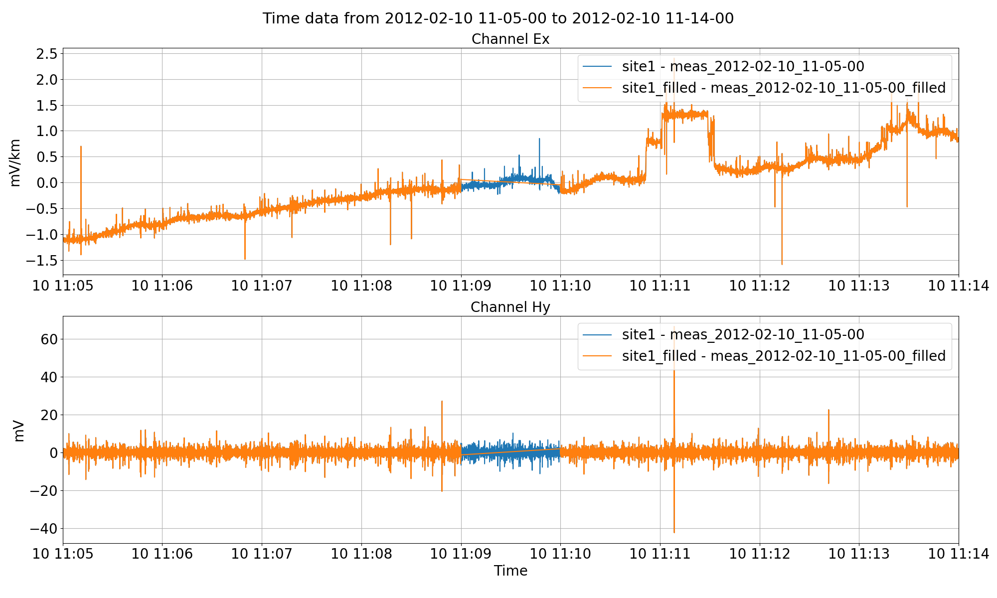
The filled time data in the new site “site1_filled”. By not removing the average throughout all the steps, the sticthed together data faithfully represents the original.
For a better understanding of the processing sequence, it is possible to look at the comments file (dataset history) of the sticthed data.
1 2 3 4 5 6 7 8 9 10 11 12 13 14 15 16 17 18 19 20 21 22 23 24 25 26 27 28 29 30 31 32 33 34 35 36 37 38 | -----------------------------
TimeData1 comments
Unscaled data 2012-02-10 11:05:00 to 2012-02-10 11:09:00 read in from measurement E:\magnetotellurics\code\resisticsdata\advanced\preprocessProject\timeData\site1\meas_2012-02-10_11-05-00, samples 0 to 983040
Sampling frequency 4096.0
Scaling channel Ex with scalar -0.000112591 to give mV
Dividing channel Ex by electrode distance 0.08 km to give mV/km
Scaling channel Ey with scalar -0.000112512 to give mV
Dividing channel Ey by electrode distance 0.091 km to give mV/km
Scaling channel Hx with scalar -0.00360174 to give mV
Scaling channel Hy with scalar -0.00360038 to give mV
Scaling channel Hz with scalar -0.0036007 to give mV
Remove zeros: False, remove nans: False, remove average: False
Time series dataset written to E:\magnetotellurics\code\resisticsdata\advanced\preprocessProject\timeData\site1_gaps\meas_2012-02-10_11-05-00_section1 on 2019-10-05 22:46:06.751226 using resistics 0.0.6.dev2
---------------------------------------------------
Unscaled data 2012-02-10 11:05:00 to 2012-02-10 11:09:00 read in from measurement E:\magnetotellurics\code\resisticsdata\advanced\preprocessProject\timeData\site1_gaps\meas_2012-02-10_11-05-00_section1, samples 0 to 983040
Sampling frequency 4096.0
Remove zeros: False, remove nans: False, remove average: False
-----------------------------
TimeData2 comments
Unscaled data 2012-02-10 11:10:00 to 2012-02-10 11:14:00 read in from measurement E:\magnetotellurics\code\resisticsdata\advanced\preprocessProject\timeData\site1\meas_2012-02-10_11-05-00, samples 1228800 to 2211840
Sampling frequency 4096.0
Scaling channel Ex with scalar -0.000112591 to give mV
Dividing channel Ex by electrode distance 0.08 km to give mV/km
Scaling channel Ey with scalar -0.000112512 to give mV
Dividing channel Ey by electrode distance 0.091 km to give mV/km
Scaling channel Hx with scalar -0.00360174 to give mV
Scaling channel Hy with scalar -0.00360038 to give mV
Scaling channel Hz with scalar -0.0036007 to give mV
Remove zeros: False, remove nans: False, remove average: False
Time series dataset written to E:\magnetotellurics\code\resisticsdata\advanced\preprocessProject\timeData\site1_gaps\meas_2012-02-10_11-05-00_section2 on 2019-10-05 22:46:06.814273 using resistics 0.0.6.dev2
---------------------------------------------------
Unscaled data 2012-02-10 11:10:00 to 2012-02-10 11:14:00 read in from measurement E:\magnetotellurics\code\resisticsdata\advanced\preprocessProject\timeData\site1_gaps\meas_2012-02-10_11-05-00_section2, samples 0 to 983040
Sampling frequency 4096.0
Remove zeros: False, remove nans: False, remove average: False
-----------------------------
Gap filled from 2012-02-10 11:09:00.000244 to 2012-02-10 11:09:59.999756
Time series dataset written to E:\magnetotellurics\code\resisticsdata\advanced\preprocessProject\timeData\site1_filled\meas_2012-02-10_11-05-00_filled on 2019-10-05 22:46:58.830430 using resistics 0.0.6.dev2
---------------------------------------------------
|
Complete example scripts
For the purposes of clarity, the complete example scripts are provided below.
Project create:
1 2 3 4 5 | from datapaths import preprocessPath
from resistics.project.io import newProject
refTime = "2012-02-10 00:00:00"
newProject(preprocessPath, refTime)
|
Data resampling:
1 2 3 4 5 6 7 8 9 10 11 12 13 14 15 16 17 18 19 20 21 22 23 24 25 26 27 28 29 30 31 | from datapaths import preprocessPath, preprocessImages
from resistics.project.io import loadProject
proj = loadProject(preprocessPath)
proj.printInfo()
from resistics.common.plot import plotOptionsTime, getPresentationFonts
plotOptions = plotOptionsTime(plotfonts=getPresentationFonts())
# resample to 1024 Hz and save in new site
from resistics.project.time import preProcess

preProcess(
    proj, sites="site1", resamp={4096: 1024}, outputsite="site1_resample", prepend=""
)
proj.refresh()
proj.printInfo()

# let's view the time series
from resistics.project.time import viewTime

fig = viewTime(
    proj,
    "2012-02-10 11:05:00",
    "2012-02-10 11:05:03",
    sites=["site1", "site1_resample"],
    chans=["Hx", "Hy", "Hz"],
    show=False,
    plotoptions=plotOptions,
)
fig.savefig(preprocessImages / "viewTimeResample.png")
|
Scaling, polarity reversal, normalising:
1 2 3 4 5 6 7 8 9 10 11 12 13 14 15 16 17 18 19 20 21 22 23 24 25 26 27 28 29 30 31 32 33 34 35 36 37 38 39 40 41 42 43 44 45 46 47 48 49 50 51 52 53 54 55 56 57 58 59 60 61 62 63 64 65 66 67 68 69 70 71 72 73 74 75 | from datapaths import preprocessPath, preprocessImages
from resistics.project.io import loadProject
proj = loadProject(preprocessPath)
proj.printInfo()
from resistics.common.plot import plotOptionsTime, getPresentationFonts
plotOptions = plotOptionsTime(plotfonts=getPresentationFonts())
# polarity reverse the Ey channel
from resistics.project.time import preProcess, viewTime

preProcess(
    proj,
    sites="site1",
    polreverse={"Ey": True},
    outputsite="site1_polreverse",
    prepend="",
)
proj.refresh()
proj.printInfo()

fig = viewTime(
    proj,
    "2012-02-10 11:05:00",
    "2012-02-10 11:05:01",
    sites=["site1", "site1_polreverse"],
    chans=["Ex", "Ey"],
    show=False,
    plotoptions=plotOptions,
)
fig.savefig(preprocessImages / "viewTimePolarityReversal.png")
preProcess(
    proj,
    sites="site1",
    scale={"Ex": -2, "Ey": 0.5},
    outputsite="site1_scale",
    prepend="",
)
proj.refresh()
proj.printInfo()

fig = viewTime(
    proj,
    "2012-02-10 11:05:00",
    "2012-02-10 11:05:01",
    sites=["site1", "site1_scale"],
    chans=["Ex", "Ey"],
    show=False,
    plotoptions=plotOptions,
)
fig.savefig(preprocessImages / "viewTimeScale.png")
# normalisation
preProcess(
proj,
sites="site1",
normalise=True,
outputsite="site1_norm",
prepend="",
)
proj.refresh()
proj.printInfo()
fig = viewTime(
proj,
"2012-02-10 11:05:00",
"2012-02-10 11:05:01",
sites=["site1", "site1_norm"],
chans=["Ex", "Ey"],
show=False,
plotoptions=plotOptions,
)
fig.savefig(preprocessImages / "viewTimeNorm.png")
|
Filtering and calibrating:
1 2 3 4 5 6 7 8 9 10 11 12 13 14 15 16 17 18 19 20 21 22 23 24 25 26 27 28 29 30 31 32 33 34 35 36 37 38 39 40 41 42 43 44 45 46 47 48 49 50 51 52 53 54 55 56 57 58 59 60 61 62 63 64 65 66 67 68 69 70 71 72 73 74 75 76 77 78 79 80 81 82 83 84 85 86 87 88 89 90 91 92 93 94 95 96 97 98 | from datapaths import preprocessPath, preprocessImages
from resistics.project.io import loadProject
proj = loadProject(preprocessPath)
proj.printInfo()
from resistics.common.plot import plotOptionsTime, getPresentationFonts
plotOptions = plotOptionsTime(plotfonts=getPresentationFonts())
# resample to 1024 Hz and save in new site
from resistics.project.time import preProcess, viewTime
preProcess(
proj, sites="site1", filter={"lpfilt": 32}, outputsite="site1_lowpass", prepend=""
)
proj.refresh()
proj.printInfo()
fig = viewTime(
proj,
"2012-02-10 11:05:00",
"2012-02-10 11:05:03",
sites=["site1", "site1_lowpass"],
chans=["Hx", "Hy", "Hz"],
show=False,
plotoptions=plotOptions,
)
fig.savefig(preprocessImages / "viewTimeLowpass.png")
preProcess(
proj, sites="site1", filter={"hpfilt": 512}, outputsite="site1_highpass", prepend=""
)
proj.refresh()
proj.printInfo()
fig = viewTime(
proj,
"2012-02-10 11:05:00",
"2012-02-10 11:05:03",
sites=["site1", "site1_highpass"],
chans=["Hx", "Hy", "Hz"],
show=False,
plotoptions=plotOptions,
)
fig.savefig(preprocessImages / "viewTimeHighpass.png")
preProcess(
proj,
sites="site1",
filter={"bpfilt": [100, 2000]},
outputsite="site1_bandpass",
prepend="",
)
proj.refresh()
proj.printInfo()
fig = viewTime(
proj,
"2012-02-10 11:05:00",
"2012-02-10 11:05:03",
sites=["site1", "site1_bandpass"],
chans=["Hx", "Hy", "Hz"],
show=False,
plotoptions=plotOptions,
)
fig.savefig(preprocessImages / "viewTimeBandpass.png")
preProcess(proj, sites="site1", notch=[50], outputsite="site1_notch", prepend="")
proj.refresh()
proj.printInfo()
fig = viewTime(
proj,
"2012-02-10 11:05:00",
"2012-02-10 11:05:03",
sites=["site1", "site1_notch"],
chans=["Hx", "Hy", "Hz"],
show=False,
plotoptions=plotOptions,
)
fig.savefig(preprocessImages / "viewTimeNotch.png")
preProcess(
    proj, sites="site1", calibrate=True, outputsite="site1_calibrate", prepend=""
)
proj.refresh()
proj.printInfo()

fig = viewTime(
    proj,
    "2012-02-10 11:05:00",
    "2012-02-10 11:05:03",
    sites=["site1", "site1_calibrate"],
    chans=["Ex", "Hx"],
    show=False,
    plotoptions=plotOptions,
)
fig.savefig(preprocessImages / "viewTimeCalibrate.png")
|
Gap filling:
1 2 3 4 5 6 7 8 9 10 11 12 13 14 15 16 17 18 19 20 21 22 23 24 25 26 27 28 29 30 31 32 33 34 35 36 37 38 39 40 41 42 43 44 45 46 47 48 49 50 51 52 53 54 55 56 57 58 59 60 61 62 63 64 65 66 67 68 69 70 71 72 73 74 75 76 77 78 79 80 81 82 83 84 85 86 87 88 89 90 91 92 93 94 95 96 97 98 99 100 101 102 103 104 | from datapaths import preprocessPath, preprocessImages
from pathlib import Path
from resistics.project.io import loadProject
proj = loadProject(preprocessPath)
proj.printInfo()
from resistics.common.plot import plotOptionsTime, getPresentationFonts
plotOptions = plotOptionsTime(plotfonts=getPresentationFonts())
from resistics.time.reader_ats import TimeReaderATS

site1 = proj.getSiteData("site1")
readerATS = TimeReaderATS(site1.getMeasurementTimePath("meas_2012-02-10_11-05-00"))
# headers of recording
headers = readerATS.getHeaders()
chanHeaders, chanMap = readerATS.getChanHeaders()
# separate out two datasets
timeOriginal1 = readerATS.getPhysicalData(
    "2012-02-10 11:05:00", "2012-02-10 11:09:00", remaverage=False
)
timeOriginal2 = readerATS.getPhysicalData(
    "2012-02-10 11:10:00", "2012-02-10 11:14:00", remaverage=False
)

from resistics.time.writer_internal import TimeWriterInternal

# create a new site
proj.createSite("site1_gaps")
proj.refresh()
writer = TimeWriterInternal()
writer.setOutPath(
    Path(proj.timePath, "site1_gaps", "meas_2012-02-10_11-05-00_section1")
)
writer.writeData(headers, chanHeaders, timeOriginal1, physical=True)
writer.setOutPath(
    Path(proj.timePath, "site1_gaps", "meas_2012-02-10_11-05-00_section2")
)
writer.writeData(headers, chanHeaders, timeOriginal2, physical=True)

from resistics.project.time import viewTime

# now view time
fig = viewTime(
    proj,
    "2012-02-10 11:05:00",
    "2012-02-10 11:14:00",
    sites=["site1", "site1_gaps"],
    filter={"lpfilt": 16},
    chans=["Ex", "Hy"],
    show=False,
    plotoptions=plotOptions,
)
fig.savefig(preprocessImages / "viewTimeGaps.png")
from resistics.time.reader_internal import TimeReaderInternal

siteGaps = proj.getSiteData("site1_gaps")
readerSection1 = TimeReaderInternal(
    siteGaps.getMeasurementTimePath("meas_2012-02-10_11-05-00_section1")
)
timeData1 = readerSection1.getPhysicalSamples(remaverage=False)
timeData1.printInfo()

readerSection2 = TimeReaderInternal(
    siteGaps.getMeasurementTimePath("meas_2012-02-10_11-05-00_section2")
)
timeData2 = readerSection2.getPhysicalSamples(remaverage=False)
timeData2.printInfo()
from resistics.time.interp import fillGap

timeDataFilled = fillGap(timeData1, timeData2)
timeDataFilled.printInfo()
samplesToView = 14 * 60 * 4096
fig = timeDataFilled.view(sampleStop=samplesToView, chans=["Ex", "Hy"])
fig.savefig(preprocessImages / "timeDataFilled.png")
# create a new site to write out to
proj.createSite("site1_filled")
proj.refresh()
# use channel headers from one of the datasets, stop date will be automatically amended
writer = TimeWriterInternal()
writer.setOutPath(
    Path(proj.timePath, "site1_filled", "meas_2012-02-10_11-05-00_filled")
)
headers = readerSection1.getHeaders()
chanHeaders, chanMap = readerSection1.getChanHeaders()
writer.writeData(headers, chanHeaders, timeDataFilled, physical=True)
proj.refresh()
# now view time
fig = viewTime(
    proj,
    "2012-02-10 11:05:00",
    "2012-02-10 11:14:00",
    sites=["site1", "site1_filled"],
    filter={"lpfilt": 16},
    chans=["Ex", "Hy"],
    show=False,
    plotoptions=plotOptions,
)
fig.savefig(preprocessImages / "viewTimeGapsFilled.png")
|